Engine Performance Analysis using Python: Data Parsing and Graphical Representation

Aim: Performing data Analysis on Engine Performance Data using PYTHON.

Objective: To perform following:

1. Demonstrating File parsing using Python
2. Plotting various graphs
3. Calculating Area Under Curve
4. Calculate engine performance Characteristics

Problem Statement:

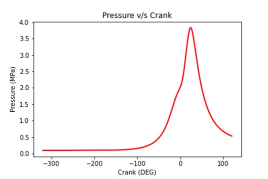
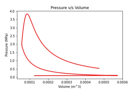
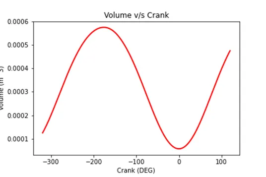
1. Data visualizer: Your script should take column numbers as the input and plot the respective columns as separate image.
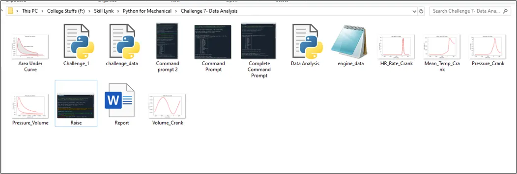
   • Each file should be saved by the name of the column. The plot labels should be extracted from the file.
   • If, I request for a plot between column 1 (crank angle) and column 8(volume), then the label information should automatically be extracted and must appear as labels in the plots.
   • THIS SHOULD NOT BE DONE MANUALLY.

2. Compatibility check:
   • You code should exit gracefully, if a non-compatible file is provided as an input.
   • It should say something like "File not recognized. Please provide a valid CONVERGE output file".
3. Basic performance calculation
   • Calculate the area under the P-V diagram. Pis in column 2 and V is in column 8.
   • Calculate the power output of this engine. Assume that RPM is 1500.
   • This engine consumed 20 micro grams of fuel (per 1 stroke cycle). Calculate its specific fuel consumption.

Theory:

The engine performance is indicated by the term efficiency. Five important engine efficiencies and other related engine performance parameters are:

1. Indicated thermal Efficiency
2. Brake thermal Efficiency
3. Mechanical Efficiency
4. Volumetric efficiency
5. Relative efficiency or Efficiency ratio
6. Mean Effective Pressure
7. Specific Power output
8. Specific Fuel Consumption
9. Inlet-valve Mach index
10. Fuel-air or Air-fuel ratio
11. Calorific value of fuel

Out of these parameters as we just need to calculate the Power and Brake Specific fuel consumption, so the necessary equations related to these parameters are as shown below:

`Power="Work Done by Engine"×n` Where n is the number of explosions per minute. For 2 stroke engines `n=N` which is the rpm of the engine while for 4 stroke engines, `n=N/2`

4 stroke Diesel Engine has been considered for the analysis, So `Power="Work Done"×N/2= J/(rev)×(rev)/(sec)="Watts"`

Specific Fuel Consumption: The fuel consumption characteristics of an engine are generally expressed in terms of specific fuel consumption in kilograms of fuel per kilowatt-hour. It is an important parameter that reflects how good the engine performance is. It is inversely proportional to the thermal efficiency of the engine.

`"sfc"=("Fuel consumption per unit time")/(Power)= ((kg)/(hr))/(kW)=(kg)/(kw-hr)`

Area under the Curve was calculated by using Simpson's rule.

Solution with Program Explanation

Program1: For data Visualiser and Compatibility Check

1. First the necessary libraries were imported which were pyplot, scipy, numpy matplotlib.patches, tabulate.
2. A display heading was printed using print
3. Using input command, the data file was imported and stored in a variable named filename.
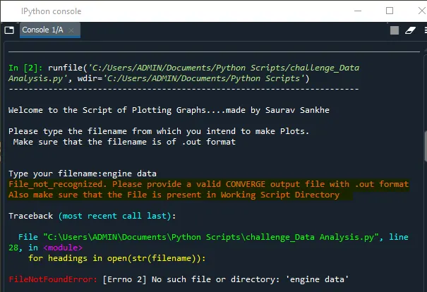
4. Then in order to perform Compatibility check, try and except raise condition was used that provided customised error generation script. In order to check this condition, incorrect file name was provided which in turn raised the following error while execution: "File not recognized. Please provide a valid CONVERGE output file". (See figure 2 of output)
5. In order to extract the heading from the file , for loop was implemented along with an if condition which extracted the headings and stored in their respective variable names (columns, prop and units), where column indices were stored in column, Properties were stored in Prop and units were stored in units.
6. As the loops reads the file line by line, as one line was read, it was split into an array of strings using split() command and these elements were stored in their corresponding variables with list data type.
7. In order to print the column indices with its corresponding properties, first the column and Prop variable elements were paired using zip() command and then it were displayed as a table in the command prompt using tabulate function which was imported from tabulate ref[3] ref[4]
8. Then the inputs were asked from the user for which he/she intend to make a plot.
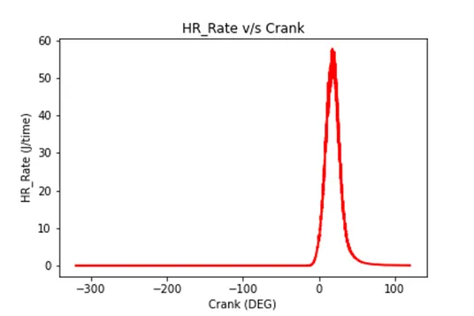
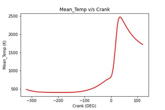
9. Finally the graphs were plotted using plot() command which was imported from the matplotlib.pyplot library.
10. As the chart title and the axis labels depend upon the user inputs, the format was coded accordingly.
11. Finally the plot was saved with the name corresponding to the column indices properties using savefig() command.

Program

# =============================================================================
# 	Data Analysis using Python
# 	by Saurav Sankhe
# =============================================================================

# Importing libraries
import matplotlib.pyplot as plt 
from scipy import integrate
import numpy as np
from matplotlib.patches import Polygon
from tabulate import tabulate

# Heading Display
print('-----------------------------------------------------------------------n')
print('Welcome to the Script of Plotting Graphs....made by Saurav Sankhen')
print('Please type the filename from which you intend to make Plots.n Make sure that the filename is of .out formatn')

# Raising Error for Incorrect Filename
filename = input('Type your filename:')

try:
	File = open(str(filename))
except:
	print('File_not_recognized. Please provide a valid CONVERGE output file with .out formatn'
       'Also make sure that the File is present in Working Script Directoryn')
 
# Reading Header Files
head = []

for headings in open(str(filename)):
	if '#' in headings:
		head.append(headings)
	    
column = head[1].split()[2:-1]
Prop = head[2].split()[1:-1]
units = head[3].split()[1:-1]

# =============================================================================
# Combining Column No and Properties In order to display in the table
# Here tabulate library was installed and imported
# Link to this library has been mentioned in the references section
# =============================================================================

Combine = list(zip(column,Prop))
headers = ['Column No','Property']
print('n')
print('Following are the Properties with corresponding Column Indices in the file')
print('Type any Two Indices to plot their graphs')
print(tabulate(Combine,headers,tablefmt="github"))

# Getting User Inputs to plot the data
X = input('Provide the Column Number from above table for your X data:')
Y = input('Provide the Column Number from above table for your Y data:')

X = int(X)		# Converting User Inputs into Integers
Y = int(Y)

X_data = []
Y_data = []
# Reading Actual Data Files
for line in open(filename):
	if '#' not in line:
		X_data.append(float(line.split()[X-1]))
		Y_data.append(float(line.split()[Y-1]))

# =============================================================================
# Plotting the Graphs
# =============================================================================
plt.plot(X_data,Y_data,linewidth=2,color='red')
plt.xlabel(Prop[X-1]+' '+units[X-1])
plt.ylabel(Prop[Y-1]+' '+units[Y-1])
plt.title(Prop[Y-1]+' v/s '+Prop[X-1])
savefile = Prop[Y-1]+'_'+Prop[X-1]+'.png'
plt.savefig(savefile)
print('n')
print('Your Graph of '+ Prop[Y-1]+' v/s '+Prop[X-1]+' has been saved in your current directory' )

Output:

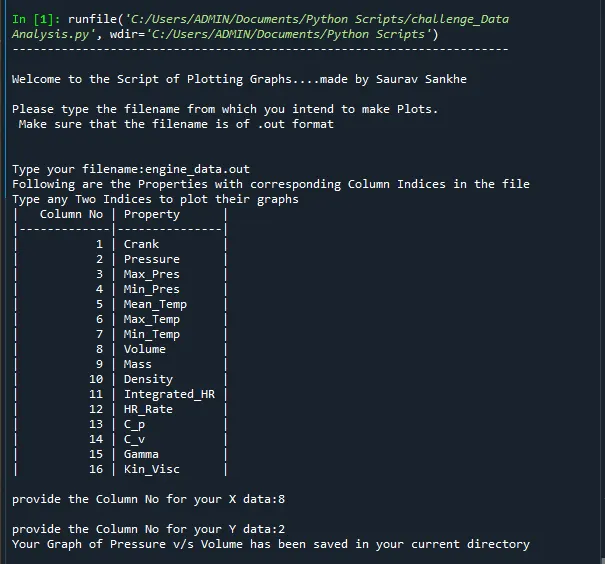
Compatibility Check (See highlighted Orange Font)

Plots

Screenshot for Saved Filenames

Program 2: Basic performance calculation

1. All the above-mentioned steps were implanted and further the code was added in it by starting with calculating the area under the curve.
2. In order to calculate area under curve, integrate module was imported from scipy module that contains simps() functions that takes two inputs arguments (X_data and y_data in this case) and calculates the area under it. ref[1]
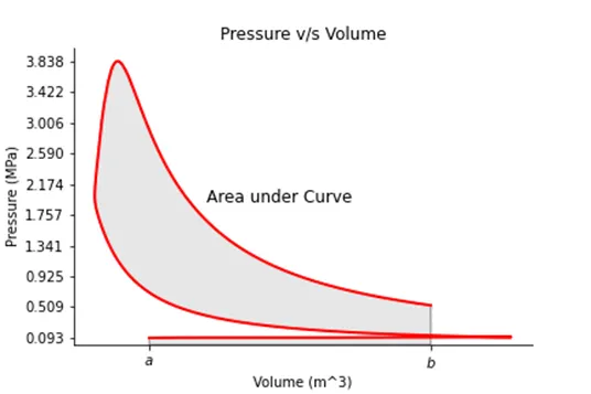
3. In order to show the shaded area of which the Area was calculated by the above said function, a polygon was fitted across the curve using polygon function imported from the patches library. ref [2]
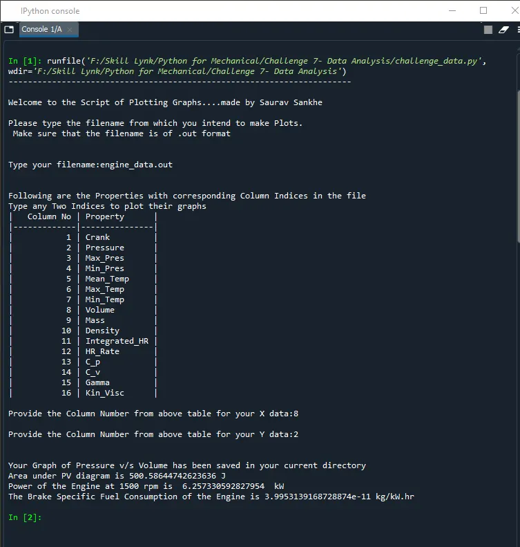
4. Finally, the poower, and specific fuel consumption were calculated using the above-mentioned formulas and were displayed on the command prompt.

Program

# =============================================================================
# 	Data Analysis using Python
# 	by Saurav Sankhe
# =============================================================================

# Importing libraries
import matplotlib.pyplot as plt 
from scipy import integrate
import numpy as np
from matplotlib.patches import Polygon
from tabulate import tabulate

# Heading Display
print('-----------------------------------------------------------------------n')
print('Welcome to the Script of Plotting Graphs....made by Saurav Sankhen')
print('Please type the filename from which you intend to make Plots.n Make sure that the filename is of .out formatn')

# Raising Error for Incorrect Filename
filename = input('Type your filename:')

try:
	File = open(str(filename))
except:
	print('File_not_recognized. Please provide a valid CONVERGE output file with .out formatn'
       'Also make sure that the File is present in Working Script Directoryn')
 
# Reading Header Files
head = []

for headings in open(str(filename)):
	if '#' in headings:
		head.append(headings)
	    
column = head[1].split()[2:-1]
Prop = head[2].split()[1:-1]
units = head[3].split()[1:-1]

# =============================================================================
# Combining Column No and Properties In order to display in the table
# Here tabulate library was installed and imported
# Link to this library has been mentioned in the references section
# =============================================================================

Combine = list(zip(column,Prop))
headers = ['Column No','Property']
print('n')
print('Following are the Properties with corresponding Column Indices in the file')
print('Type any Two Indices to plot their graphs')
print(tabulate(Combine,headers,tablefmt="github"))

# Getting User Inputs to plot the data
X = input('Provide the Column Number from above table for your X data:')
Y = input('Provide the Column Number from above table for your Y data:')

X = int(X)		# Converting User Inputs into Integers
Y = int(Y)

X_data = []
Y_data = []
# Reading Actual Data Files
for line in open(filename):
	if '#' not in line:
		X_data.append(float(line.split()[X-1]))
		Y_data.append(float(line.split()[Y-1]))

# =============================================================================
# Plotting the Graphs
# =============================================================================
plt.plot(X_data,Y_data,linewidth=2,color='red')
plt.xlabel(Prop[X-1]+' '+units[X-1])
plt.ylabel(Prop[Y-1]+' '+units[Y-1])
plt.title(Prop[Y-1]+' v/s '+Prop[X-1])
savefile = Prop[Y-1]+'_'+Prop[X-1]+'.png'
plt.savefig(savefile)
print('n')
print('Your Graph of '+ Prop[Y-1]+' v/s '+Prop[X-1]+' has been saved in your current directory' )

# =============================================================================
# Calculating Area under the Curve
# Area Under Curve was calculated using Simphson's function available in 
# Scipy integrate module
# =============================================================================
Area = integrate.simps(Y_data,X_data)
print('Area under PV diagram is '+ str(Area*1e6) + ' J')

# =============================================================================
# Plotting the Shaded Curve
# Polygon Function was used to show shaded area in the curve 
# This functionnwas available in matplotlb.patches module
# =============================================================================
a = X_data[0]
b = X_data[-1]

fig, ax = plt.subplots()
ax.plot(X_data, Y_data, 'r', linewidth=2)
ax.set_ylim(bottom=0)


verts = [(a, 0), *zip(X_data, Y_data), (b, 0)]
poly = Polygon(verts, facecolor='0.9', edgecolor='0.5')
ax.add_patch(poly)

ax.spines['right'].set_visible(False)
ax.spines['top'].set_visible(False)
ax.xaxis.set_ticks_position('bottom')

# Adding Text
ax.text((0.5*np.max(X_data)),(0.5*np.max(Y_data)), 'Area under Curve', horizontalalignment='center', fontsize=12)
ax.set_xticks((a, b))

ax.set_xticklabels(('$a$', '$b$'))
ax.set_yticks(np.linspace(np.min(Y_data),np.max(Y_data),10))
plt.xlabel(Prop[X-1]+' '+units[X-1])
plt.ylabel(Prop[Y-1]+' '+units[Y-1])
plt.title(Prop[Y-1]+' v/s '+Prop[X-1])
plt.savefig('Area Under Curve.png')
# plt.show()

# =============================================================================
# Calculating power of the Engine With N = 1500 rpm
# Power = Area*n where n = N/2 for 4 Stroke Engine
# =============================================================================

N = 1500
Power = Area*1e6*(N/(2*60))
print('Power of the Engine at '+ str(N) +' rpm'+' is ',Power*1e-3, ' kW' )

# =============================================================================
# Calculating Brake Specific Fuel Consumption (bsfc)

# bsfc = m_f/power
# =============================================================================

m = 20e-9       #20 miligrams/stroke_cyle to 20 kg/stroke_cycle
m_f = m*(N/(2*60))  # in kg/sec

bsfc = m_f/Power
print('The Brake Specific Fuel Consumption of the Engine is ' + str(bsfc) + ' kg/kW.hr' )

Output

Conclusion

1. File parsing was successfully implemented using Python. Python is a very powerful tool useful for carrying data analysis. As about 8000 lines of file was been read in only 10-20 seconds from python script.
2. Compatibility test was also successfully scripted.
3. Basic Engine performance parameters were also calculated and are documented as below

Parameter	Value
Area Under Curve	500.58644742623636 J
Power	6.257330592827954 kW
Specific Fuel Consumption	3.9953139168728874e-11 kg/kW.hr

References :

1. simps function from Scipy Library
2. Calculating Area Under Curve
3. Tabulate library
4. Basic Commands used from Python