Week 6: Conjugate Heat Transfer Simulation

Conjugate Heat Transfer Simulation

Aim:

Baseline configuration

• Setup a flow simulation through a pipe
• Inlet Reynolds number should be 7,000
• Turbulence modelling - K-Epsilon
• Supercycling parameters - same as in the video

Grid dependence test

• Start with an initial base grid
• Run grid dependence test on 3 grids and show that the outlet temperature converges to a particular value

Effect of supercycle stage interval

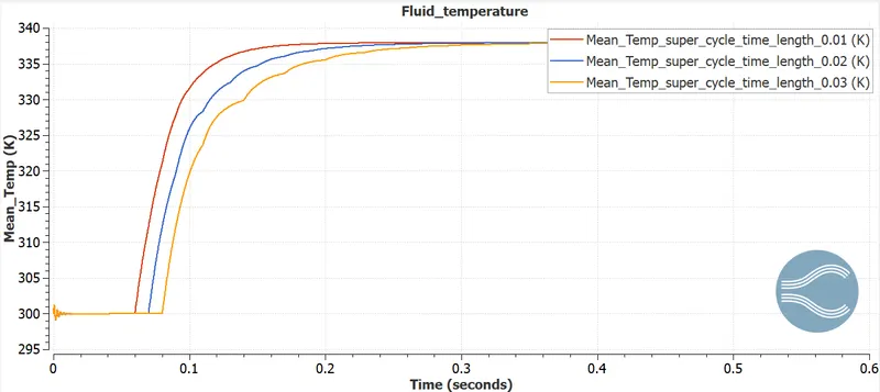
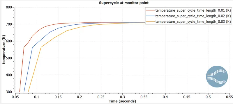
• Set supercyle stage interval to 0.01,0.02 and 0.03
• For these three values, how does the total simulation time compare against the baseline configuration

Geometry:

The geometry was imported into the converge and Cad clean up was done.

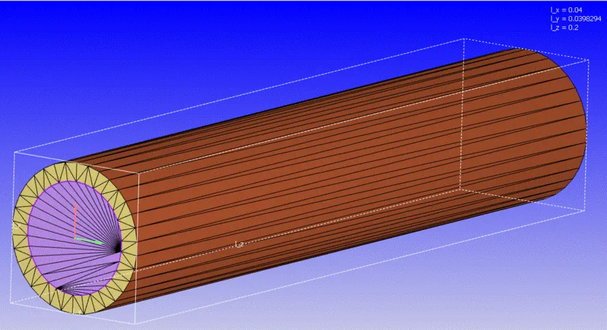
• inner radius = 0.015
• outer radius = 0.02
• length = 0.2

Case-Setup

• Application: General Flow
• Solver: Steady state solver
• Material: Air
• Solid - Aluminium
• Species: O2 and N2
• Simulation mode: Full hydrodynamic
• Simulation time parameters:
  Start time:0sec
  End time:0.5 sec
• Region & Initialization:
  Created a fluid and solid region for initializing the setup

Boundary conditions

• Inlet:
• Boundary type = inflow
• Pressure = zero gradient (Neumann boundary condition)
• Temperature = 300 K
• Velocity = 7.2877 m/s
• outlet:
• Boundary type = outflow
• Pressure = 101325 Pa
• Temperature = 300 K
• Species = air
• Solid outer wall
• Boundary type = wall with slip condition
• Wall motion type = stationary
• Temperature = -10000 w/m2 (Heat flux)
• Solid side
• Boundary type = wall with slip condition
• Wall motion type = stationary
• Temperature = zero gradient (Neumann boundary condition)
• Interface
• Boundary type = interface
• Boundary type = interface
• region 1 = Fluid region
• Stream ID = 0
• Temperature = 300 K
• Pressure = 101325 Pa
• Species = air
• region 2 = Solid region
• Stream ID = 1
• Temperature = 300 K
• Solid option - enabled
• Species = Aluminium
• Boundary type = interface
• region 1 = Fluid region
• Stream ID = 0
• Temperature = 300 K
• Pressure = 101325 Pa
• Species = air
• region 2 = Solid region
• Stream ID = 1
• Temperature = 300 K
• Solid option - enabled
• Species = Aluminium
• Turbulence Model - K epsilon
• The time interval for writing 3D output data files:=0.01
• The time interval for writing text output:1e-6 sec
• The time interval for writing restarting output:0.01
• Maximum number of restart file saved:3
• Super cycling
• Time length for cycle stage = 0.01, 0.02, 0.03.

Results

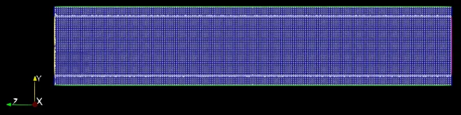
• Mesh

1. mesh size 0.004

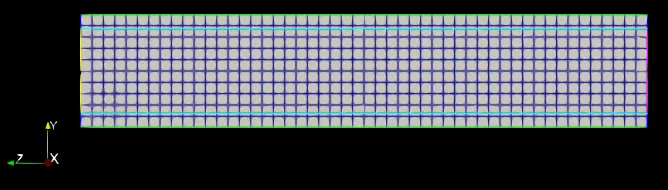
2. mesh size 0.003

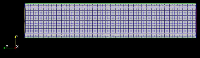
3. mesh size 0.002

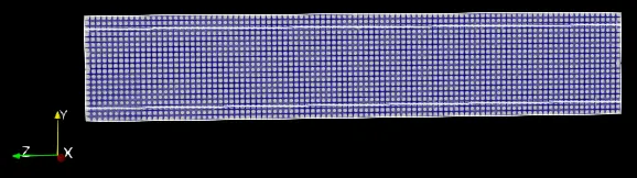
4. mesh size 0.001

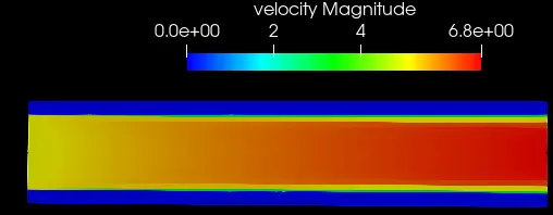
• Velocity Contours

1. mesh size 0.004

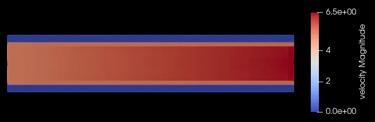
2. mesh size 0.003

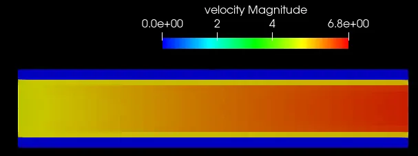
3. mesh size 0.002

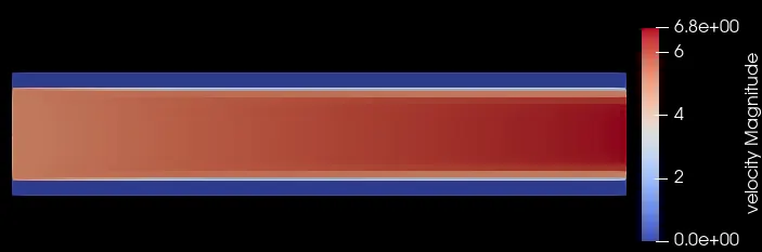
4. mesh size 0.001

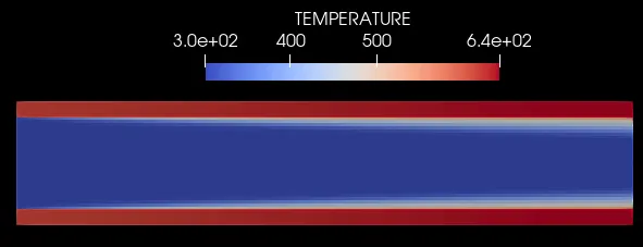
• Temperature

1. mesh size 0.004

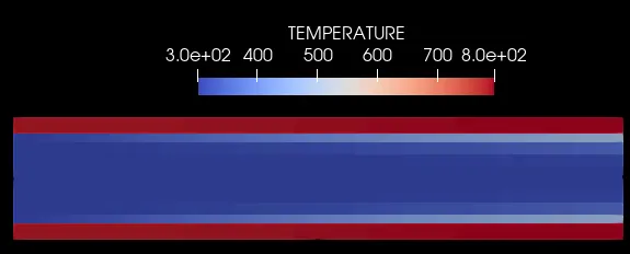
2. mesh size 0.003

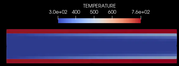
3. mesh size 0.002

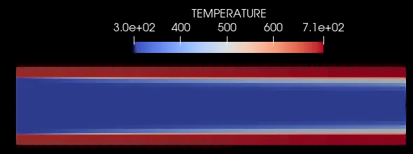
4. mesh size 0.001

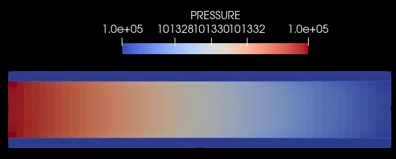
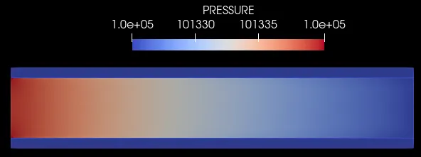
• Pressure

1. mesh size 0.004

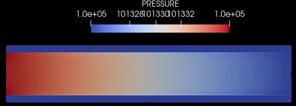
2. mesh size 0.003

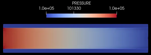
3. mesh size 0.002

4. mesh size 0.001

• Wall Y+

1. mesh size 0.003

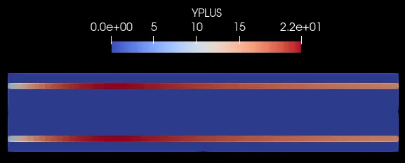
2. mesh size 0.002

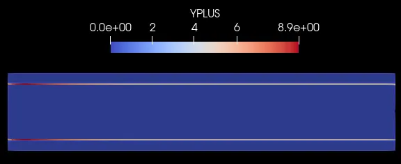
3. mesh size 0.001

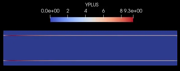
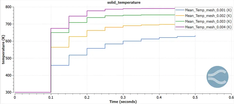
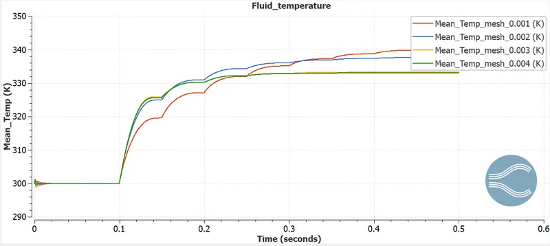
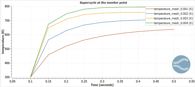
• Temperature Plots with mesh refinement

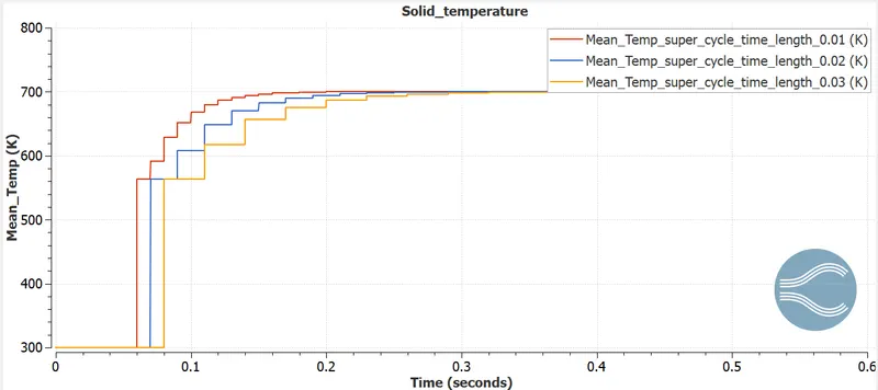
• Temperature plots with super-cycle time length variation (mesh = 0.02)

.

Conclusion

• CHT analysis is done on solid-hollow cylindrical geometry.