Week 6: Conjugate Heat Transfer Simulation

AIM: To perform Conjugate Heat Transfer flow simulation through a pipe using Converge CFD and post process the results using Paraview.

OBJECTIVE:

• • Setup a flow simulation through a pipe
  • Inlet Reynolds number should be 7,000

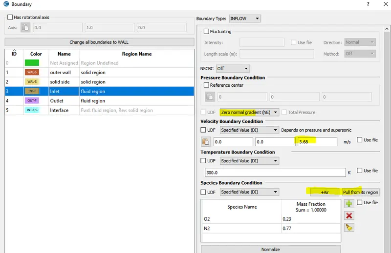
    • HINT : Use the below formula to calculate velocity for corresponding value of REYNOLD NUMBER and give DIRICHLET BC for velocity at inlet and specify the value for velocity calculated at INLET BC using below formula ,

      Re = (rho*V*D)/(Dynamic viscosity)

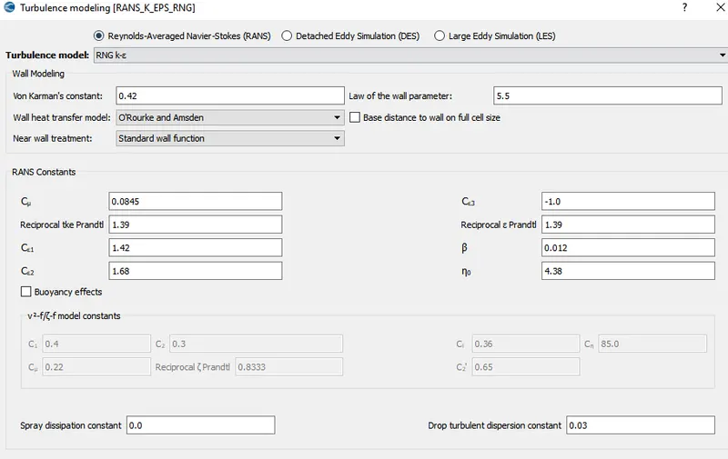
  • Turbulence modelling - K-Epsilon
  • Supercycling parameters - same as in the video

  Additional 3D outputs

  • Add Y+ to your post.in file

  Grid dependence test

  • Start with an initial base grid
  • Run grid dependence test on 3 grids and show that the outlet temperature converges to a particular value

  Effect of supercycle stage interval

  • Set supercyle stage interval to 0.01,0.02 and 0.03
  • For these three values, how does the total simulation time compare against the baseline configuratio

METHODOLOGY:

Introduction:

When multiple modes of heat transfer ie., variations of temperature within solids and fluids, due to thermal interaction between the solids and fluids are involved then the process is called Conjugate Heat Transfer.

Wall functions are useful in calculation the solutions near the wall. Y+ is a dimensionaless quantity that can be used to understand whether the mesh is coarse or fine which in turn determines the need for wall functions. The Turbulent flow have a smaller laminar region near the wall and if we are to resolve the gradients at such a small region, very small grid size is required.

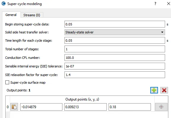
Super cycling is a method that is used to solve CHT simulations in converge. In this method solver solves the solid region and fluid region seperately. The time scale difference between both the fluid and solid regions is very high as the time required for solver to attain steady state in fluid region is very small when compared to that of solid. In supercycling, the solver of the fluid domain is paused untill the solid domain reaches steady state. This pausing is called as supercycling stage interval and it is user defined in pre processing.

Initially, for 0.1s, both the fluid domain and solid domain solvers are run. At first interval, 0.1s, the fluid solver is paused and the solid side solver is continued to run towards convergence.

PROCEDURE:

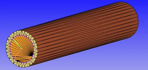
1. Geometry

Case Setup-

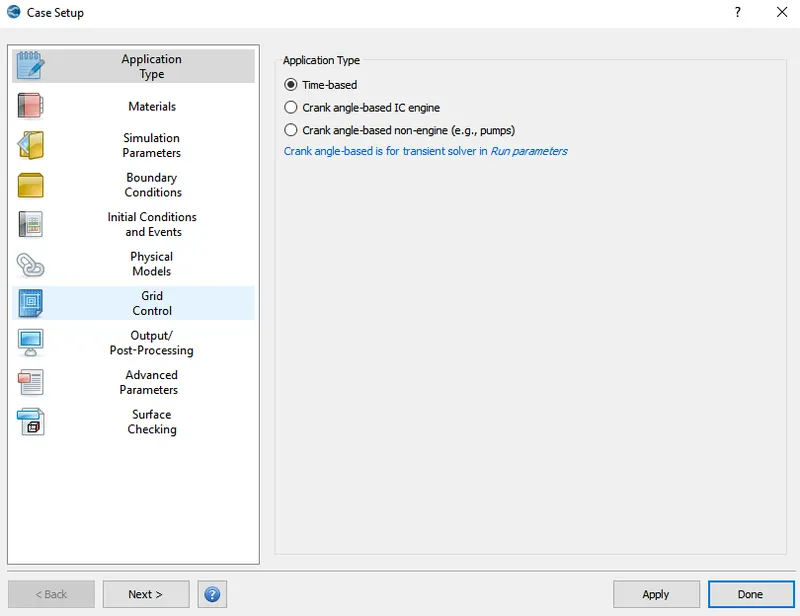
2. Application Type = Time-based

3. Materials - Predefined mixtures = Air

Select 'Gas Simulation', 'Solid simulation' and 'species'.

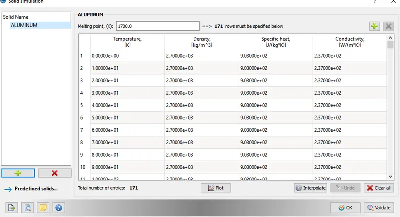
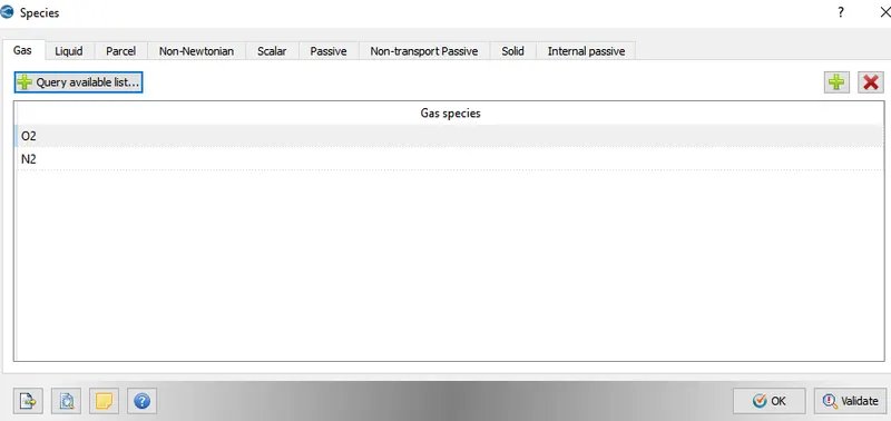
4. Simulation Parameters-

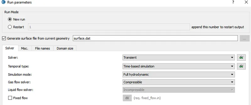
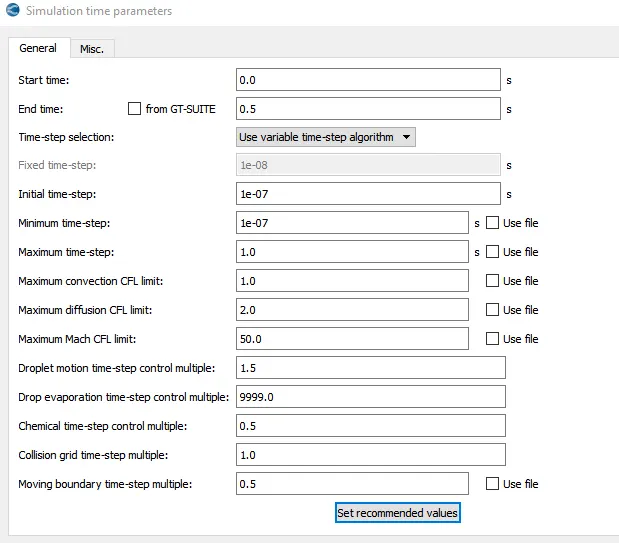
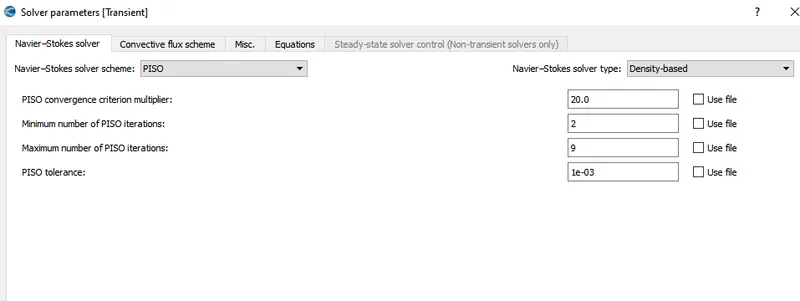
5. Boundary Conditions-

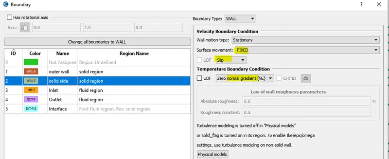
Outer Wall:

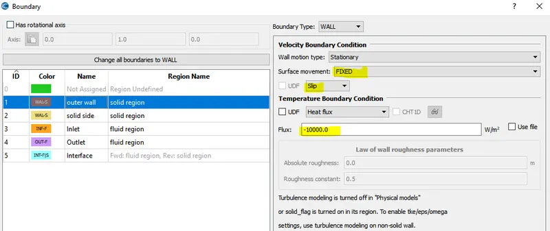
Solid side:

Inlet:

Online Calculation of Air (peacesoftware.de)
PARAMETERS	VALUE	UNIT	FORMULA
density	1.17678	kg/m^3
Reynolds Number	7000
diameter	0.03	m
Dynamic Viscosity	1.86E-05	10-6 (Pa s) or Ns/m^2
Velocity	3.681705	m/s	Re = (rho*V*D)/(Dynamic viscosity)

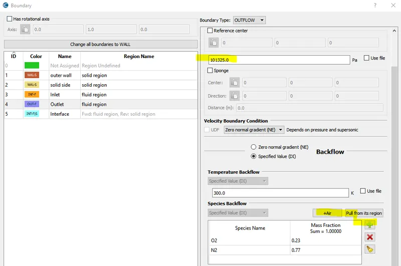
Outlet:

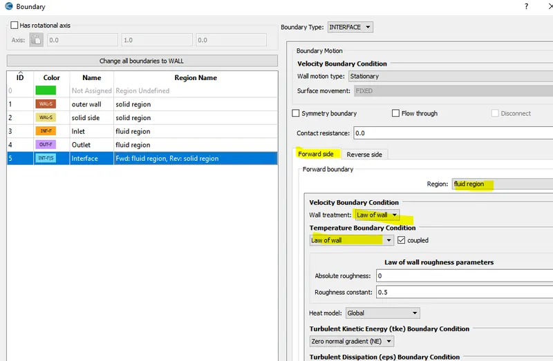
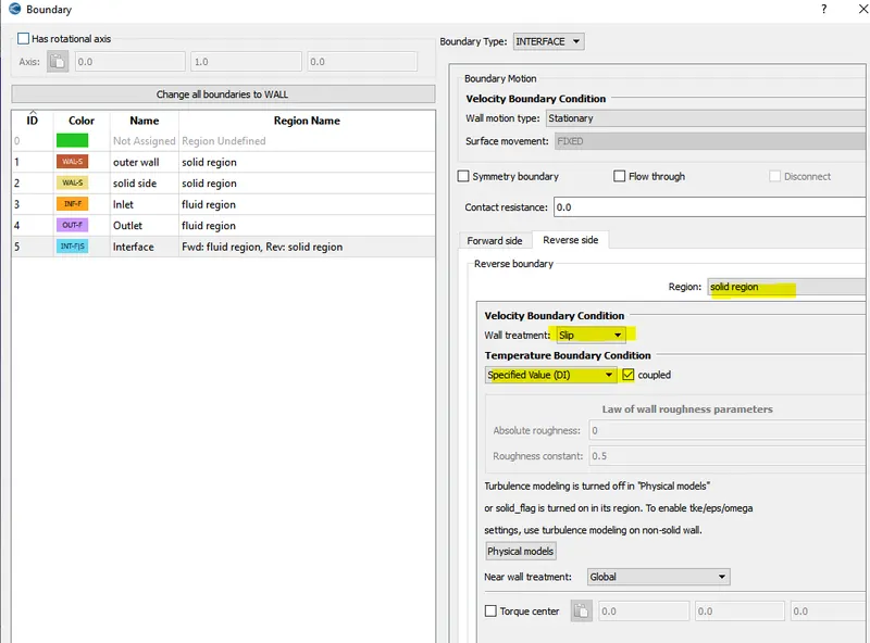
Interface:

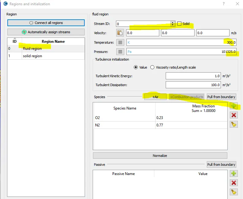
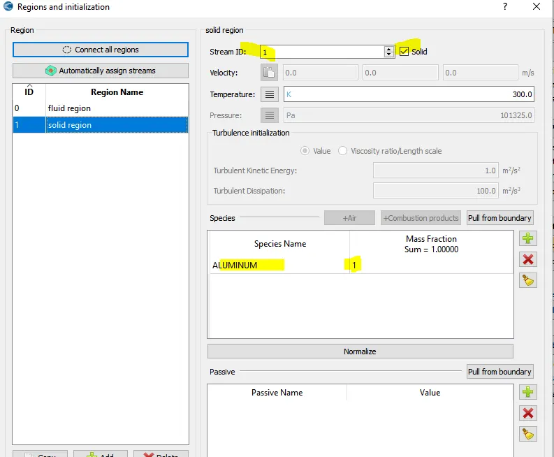
6. Initial Conditions and Events:

7. Physical Models:

Super Cycle Modeling

8. Grid Control:

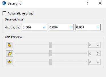
9. Post-Processing:

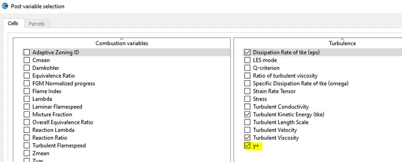
10. Output Files:

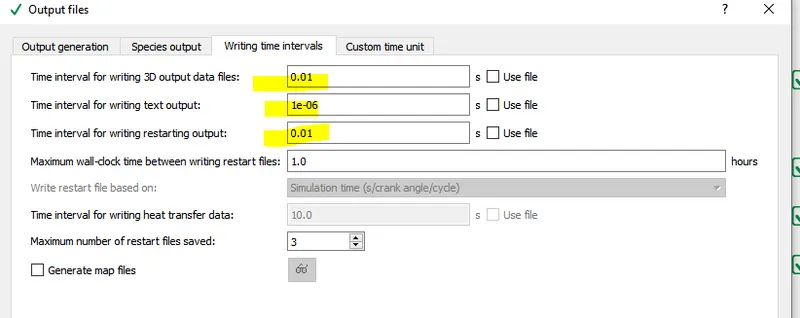
3. RESULTS AND DISCUSSION:

PLOTS and CONTOUR:

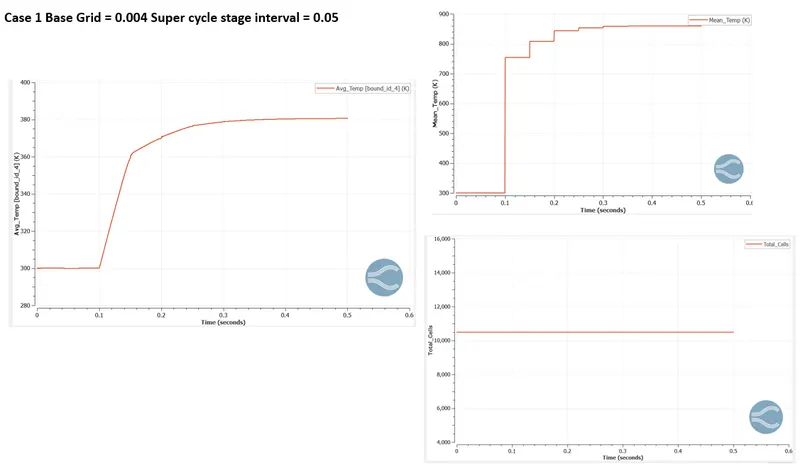
GRID DEPENDENCY TEST : (Mesh Size = 0.004, 0.003, 0.002)

Temperature Animation Link https://youtu.be/dhuhZfAAeDY

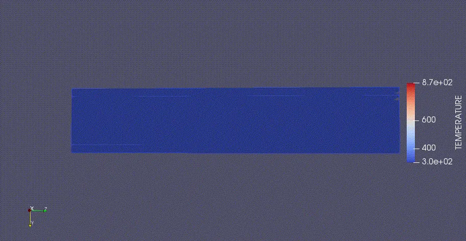
Temperature Animation Link https://youtu.be/fpRYsZqFwLY

Temperature Animation Link https://youtu.be/KmVuCtgBVSs

Inference: The following inferences were made from the above plots and contours:

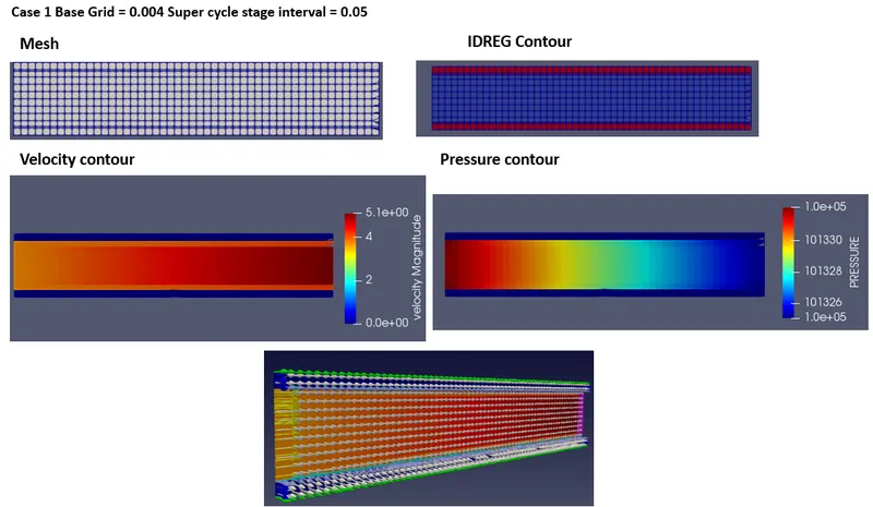
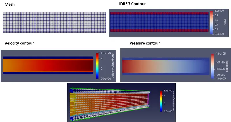
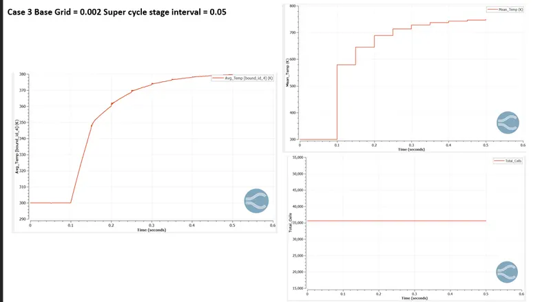
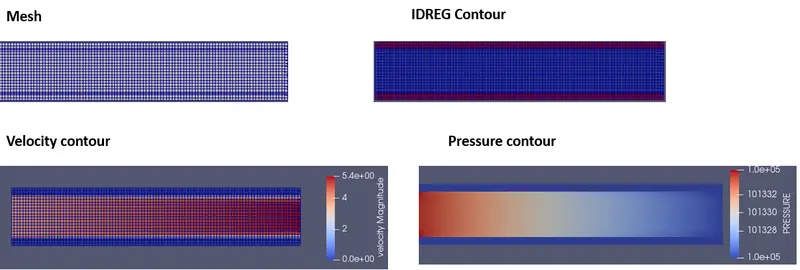
• Mesh: For a Grid Size of 0.004 the mesh is found to be too course and from grid dependency test it is clear that as the mesh size is reduced the results are accurate with increase in cell count and computation time trade off.
• IDREG Contour: It helps to differntiate the solid region from fluid region. The solid region is indicated as 1 and fluid region is represented as 0 in the contour
• Vector Contour : Velocity Vector contour confirms the direction of fluid flow.
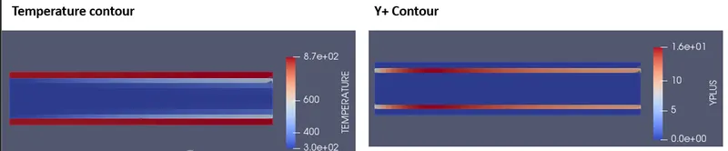
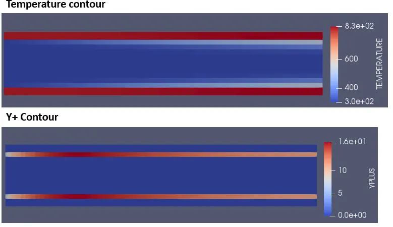
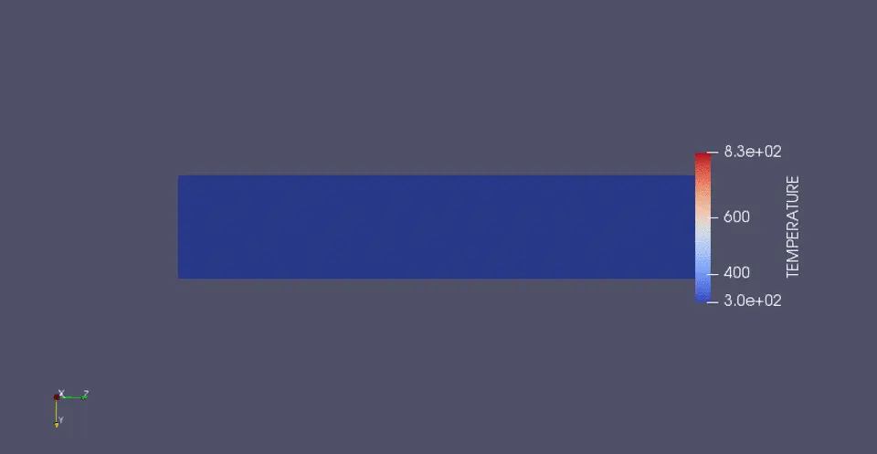
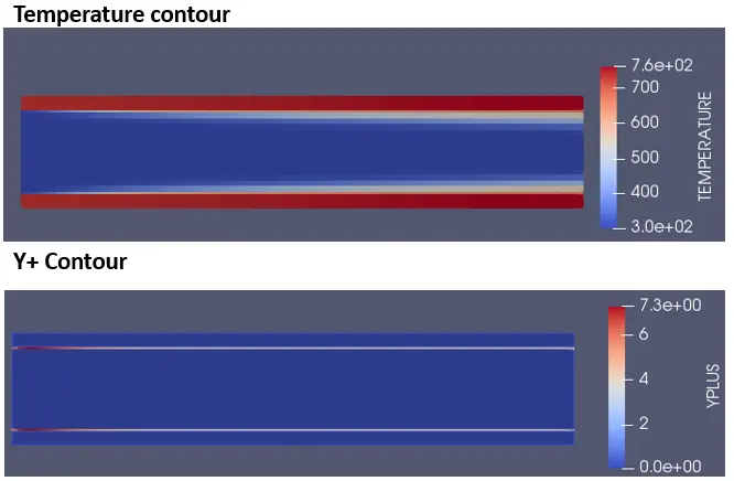
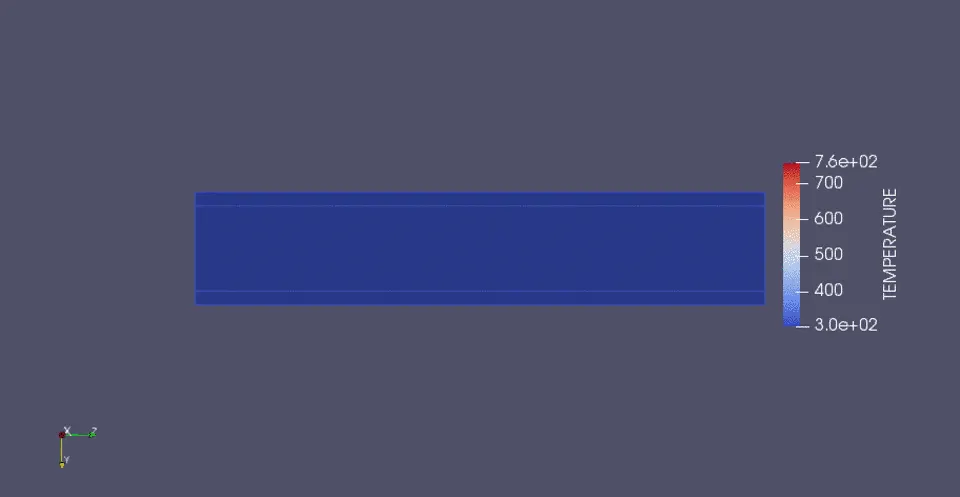
• Temperature Contour: It is envisaged from the graph that first the transfer of heat take place on the solid pipe due to heat flux source. Then by conduction, heat is transfered through the solid region and for the fluid in pipe the heat is passed on by convection. Moreover the outle temperature converges at different values for different mesh sizes.
• Y+ Contour: The y+ value is a non-dimensional quantity that is used to understand how coarse or fine a mesh is. As the mesh size decreases from 0.004 to 0.002 the Y+ value also decreases and it could be seen visually in Y+Contour.
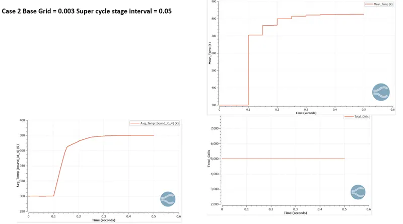
• Mean Temperature Plot: It clearly shows that the Solid region takes lot of time to attain steady state and thus time scale difference between both the fluid and solid regions is very high.
• Cell Count: As the mesh size decreases from 0.004 to 0.002 the cell count increases proportionately from 11000 to 36000 Approx.

Effect of Super Cycle Stage interval

Case 1: Gride size=0.003 and supercyle stage interval=0.01

Case 2: Gride size=0.003 and supercyle stage interval=0.02

Case 3: Gride size=0.003 and supercyle stage interval=0.03

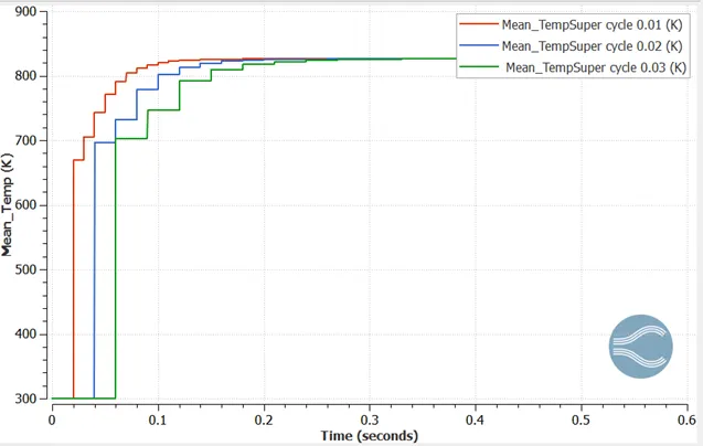
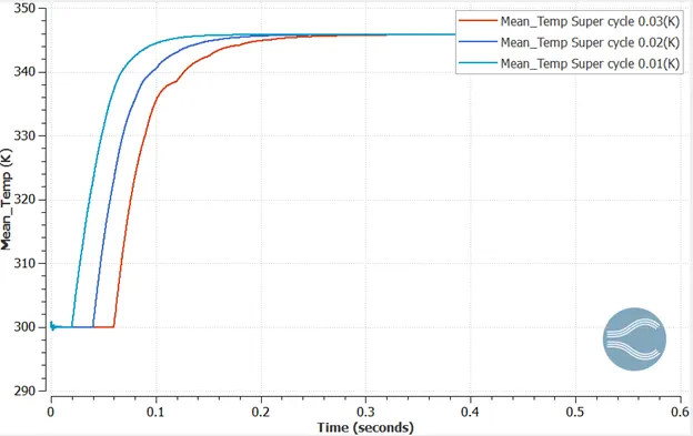
Super cycle 0.01 run time 1186 sec

Super cycle 0.02 run time 1059 sec

Super cycle 0.03 run time 893 sec

Inference: The following inferences were made from the above plots

• It is clear from the Mean Temp Vs Time Plot of fluid and solid that the time scale difference between both the fluid and solid regions is very high as the time required for solver to attain steady state in fluid region is very small when compared to that of solid.
• Supercycling interval decreases the simulation time increases

4. CONCLUSION: The study of Conjugate Heat Tranfer through a pipe using Converge CFD and Paraview was simulated successfully.