Week 6: Conjugate Heat Transfer Simulation
AIM: To perform Conjugate Heat Transfer simulation for baseline configuration, to carry out the grid dependency test on 3 grids, to analyse the effect of supercycle stage interval
Theoritical Background:
Conjugate Heat Transfer(CHT)
The term conjugate heat transfer (CHT) describes the processes which involve variations of temperature within solids and fluids, due to thermal interaction between the solids and fluids. The exchange of thermal energy between the two physical bodies is called study of Heat Transfer, the rate of transferred heat is directly proportional to the temperature difference between the bodies.
Conjugate heat transfer corresponds with the combination of heat transfer in solids and heat transfer in fluids. In solids, conduction often dominates whereas in fluids, convection usually dominates. Efficiently combining heat transfer in fluids and solids is the key to designing effective coolers, heaters, or heat exchangers. Forced convection is the most common way to achieve high heat transfer rate. In some applications, the performances are further improved by combining convection with phase change.
Heat transfer in solids and heat transfer in fluids are combined in the majority of applications. This is because fluids flow around solids or between solid walls, and because solids are usually immersed in a fluid.
Super Cycling:
It is a method used by Converge Studio in case of Conjugate Heat Transfer Problems with Solid and liquid regions. The integral problem here is that both solvers cannot run at the same speed, since soliving in the fluid domain is much faster owing to the time scale difference for heat transfer in liquids as compared to solids. This causes a problem duing the solution given that the solid side solver would not have reached a steady state or convergence in the time liquid solver does. Here the Supercycling can be used.
The primary concept behind super cycling is that the solver for the fluid domain is paused until the solver for the solid domain converges. This pausing can be done in the intervals that can be set by the user. Super cycling is only meant to speed up the simulation and if the simulation runs without supercycling, the convergence of data will take long time.
Geometry:
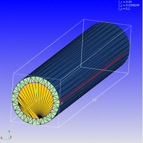
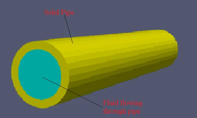
Case Setup:
1] Materials:
Gas is flowing through the pipe and outside is the metal
2] Simulation parameters
Solver: Transient
Simulation mode is full hydrodynamic and Gas flow solver is compressible
3] Simulation Time Parameters
Start Time = 0s, End Time = 0.5s, Initial and Minimum Time step = 1e-7s, Maximum Time step = 1s
4] Regions and Initialization
Grouping the boundaries to form Volumetric zones called regions. This defines the volumetric regions with initial conditions like Pressure, Velocity, Temperature and Species Concentration. Add two regions namely Fluid and Solid region.
Fluid region - velocity = [0,0,0] m/s, Stream ID = 0, Temperature = 300 K, Pressure = 101325 P, Species = Air.
Solid region - Stream ID = 1, Temperature = 300 K, Species = Alluminimu (mass fraction = 1)
5] Boundary Conditions:
We have to assign boundary conditions for different faces of Geometry as shown in the table below
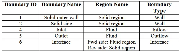
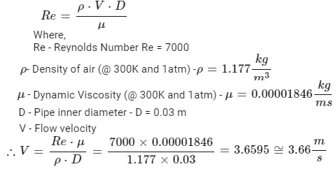
Calculation of Velocity at the Inlet boundary condition based on Reynolds number
Grid Dependency Test
Case 1A: dx =dy= dz = 0.004m, grid size
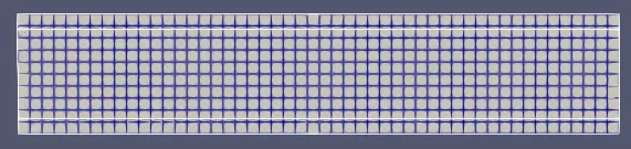
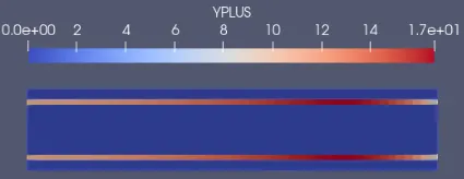
Y+ Contour
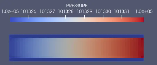
Pressure Contour
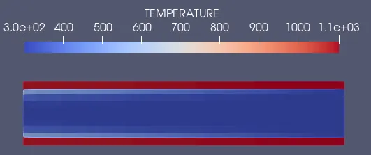
Temperature Contour
Velocity Contour
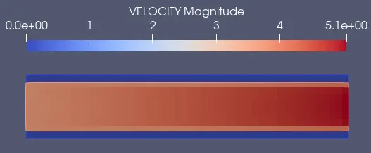
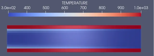
Case 1B: dx =dy= dz = 0.003m, grid size
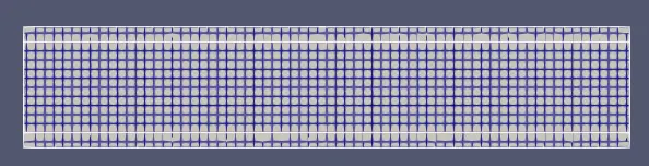
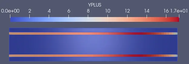
Y+ Contour
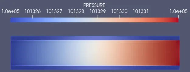
Pressure Contour
Temperature Contour
Velocity Contour
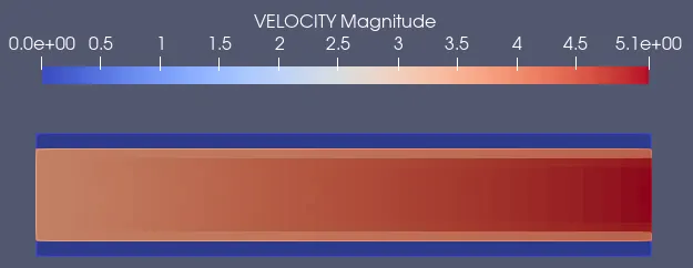
Case 1C: dx =dy= dz = 0.002m, grid size
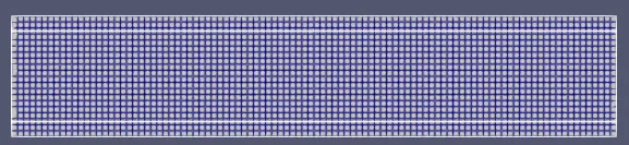
Y+ Contour
Pressure Contour
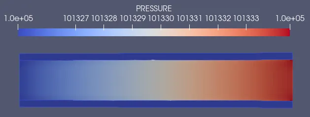
Temperature Contour
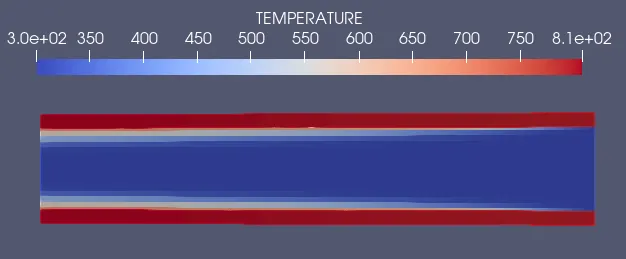
Velocity Contour
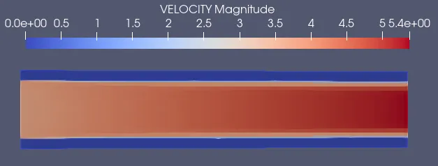
Temperature plots for different grid size
A] Fluid region
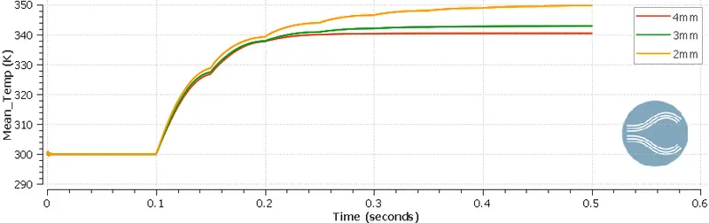
B] Solid region
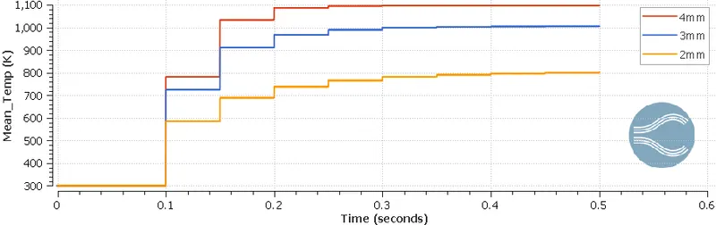
The Temperature in the Fluid region is going to be 350 K and the temperature in the Solid region is going to be 1100 K. It can be seen that the temperature changes, as the size of the grid changes. We can observe that for finer mesh the mean temperature in the solid region is low,where as in the fluid region, mean temprature is high. Here the temperatures are variant to the change in the grid size. Mesh size can be reduced further to obtain the high level of accuracy until the results become grid independent.
Effect of Supercycle Stage Interval
Case 2A: Supercyle stage interval = 0.01s
Mean Temperature in the Liquid region
Mean Temperature in the Solid region
Case 2B: Supercyle stage interval = 0.02s
Mean Temperature in the Liquid region
Mean Temperature in the Solid region
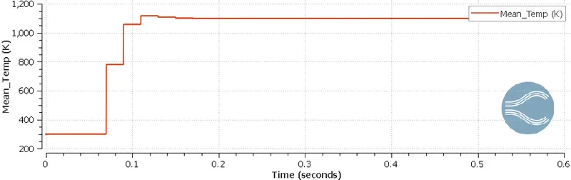
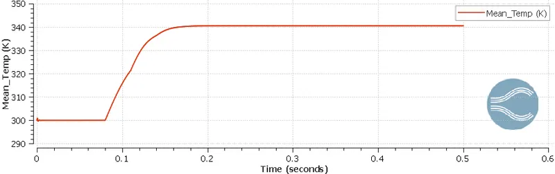
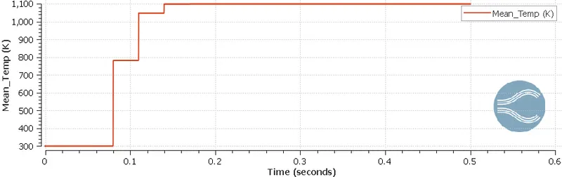
Case 2C: Supercyle stage interval = 0.03s
Mean Temperature in the Liquid region
Mean Temperature in the Solid region
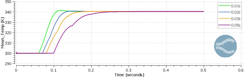
Fluid region at a mesh size = 0.004m at a Supercycle stage interval of 0.01s ,0.02s, 0.03s,0.05s
Solid region at a mesh size = 0.004m at a Supercycle stage interval of 0.01s ,0.02s, 0.03s,0.05s
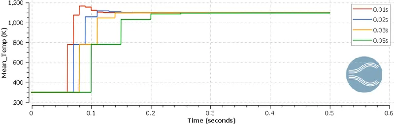
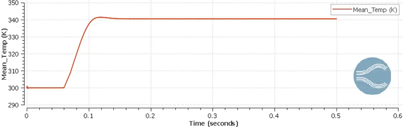
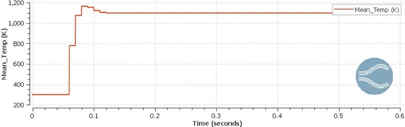
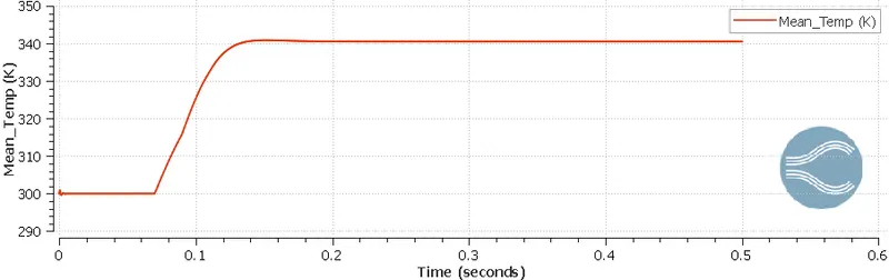
For the fluid region the curve attains convegence faster for the lower value of Supercycle stage interval. As the value of the supercycle stage interval is low, less is the time taken for processing it in cygwin when compared it with baseline configuration. Solid takes much time to heat up due to huge capacitence, hence more time is needed to increase the temperature.
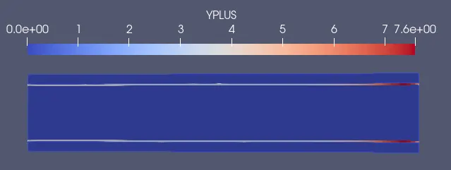
Y+ data
The y+ value is a non-dimensional term that can be used to understand how coarse or fine our grid is. This can then be used to determine if wall functions need to be used or not. Using the y+, the way in which velocity is calculated changes. The y+ value gives us an idea of where the first cell center lies. Using the y+ value, we can understand how exactly we can approach the problem.
The significance of y+:
The y+ value denotes wherein the y+ vs u+ curve we are with respect to the cell size. It is undesirable to have a cell size that leads to a y+ of between 10 to 30 since the modeling of flows transitioning from laminar to turbulent is not easy. Due to this fact, it is better to have a y+ of less than 10 meaning we'd be at the laminar region or have a y+ of greater than 30 where we can go with a wall function and still achieve results. The y+ value can be used as a marker based on which we can decide on the base grid size and make a decision based on the computing power as to whether the grid needs to be refined further or coarsened.
Y+ values for different grid size are as tabulated below
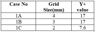
It was observed that as the grid size reduces, the Y+ value also decreases