Week 6: Conjugate Heat Transfer Simulation
Aim: Conjugate Heat Transfer Simulation.
Objectives:
- To run grid dependence test on 3 grids and to show that the outlet temperature converges to a particular value.
- To show the effect of supercycle stage interval
- To set the supercycle stage interval to 0.01,0.02 and 0.03, for these three values, how does the total simulation time compare against the baseline configuration.
Introduction:
The term conjugate heat transfer (CHT) is used to describe processes which involve variations of temperature within solids and fluids, due to thermal interaction between the solids and fluids.
The exchange of thermal energy between the two physical bodies is called the study of Heat Transfer, the rate of transferred heat is directly proportional to the temperature difference between the bodies. A typical example is the heating or cooling of a solid object by the flow of air in which it is immersed and some other example includes conduction through solids, free and forced convection in the gases/fluids and thermal radiation.
Modes of heat transfer
-
Conduction: diffusion of heat due to temperature gradients. A measure of the amount of conduction for a given gradient is heat conductivity.
-
Convection: when the heat is carried away by moving fluid. The flow can either be caused by external influences, forced convection; or by buoyancy forces, natural convection. Convective heat transfer is tightly coupled to the fluid flow solution.
-
Radiation: transfer of energy by electromagnetic waves between surfaces with different temperatures, separated by a medium that is at least partially transparent to the (infrared) radiation. Radiation is especially important at high temperatures, e.g. during combustion processes, but can also have a measurable effect at room temperatures.
Theory:
Conjugate heat transfer corresponds with the combination of heat transfer in solids and heat transfer in fluids. In solids, conduction often dominates whereas, in fluids, convection usually dominates. Efficiently combining heat transfer in fluids and solids is the key to designing effective coolers, heaters, or heat exchangers. Forced convection is the most common way to achieve a high heat transfer rate. In some applications, the performances are further improved by combining convection with phase change (for example liquid water to vapour phase change).
Heat transfer in solids and heat transfer in fluids are combined in the majority of applications. This is because fluids flow around solids or between solid walls and because solids are usually immersed in a fluid.
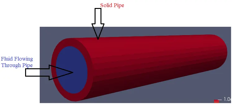
The conjugate heat transfer methods have become a more powerful tool for modelling and investigating nature phenomena and engineering systems in different areas ranging from aerospace and nuclear reactors to thermal goods treatment and food processing, from complex procedures in medicine to atmosphere/ocean thermal interaction in meteorology, and from relatively simple units to multistage, nonlinear processes.
Geometry Setup:
Creating Geometry:
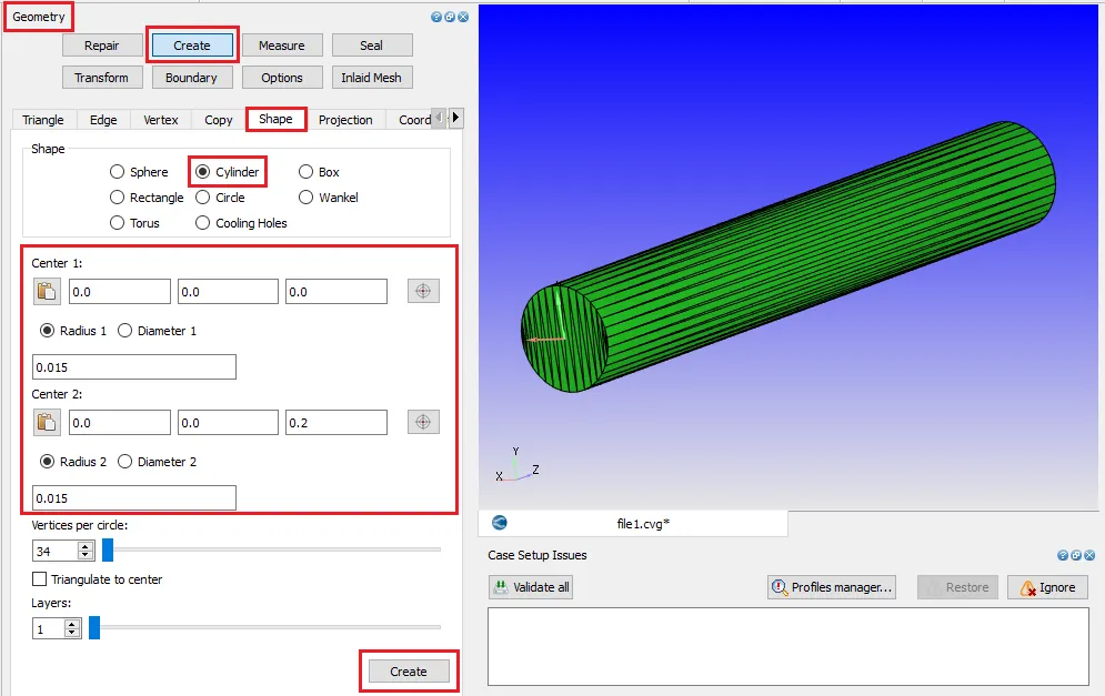
1. Creating Pipe:
Create> Shape> Cylinder> Center 1 and Center 2> Radius=0.015> Create
Similarly,
Create> Shape> Cylinder> Center 1 and Center 2> Radius=0.02> Create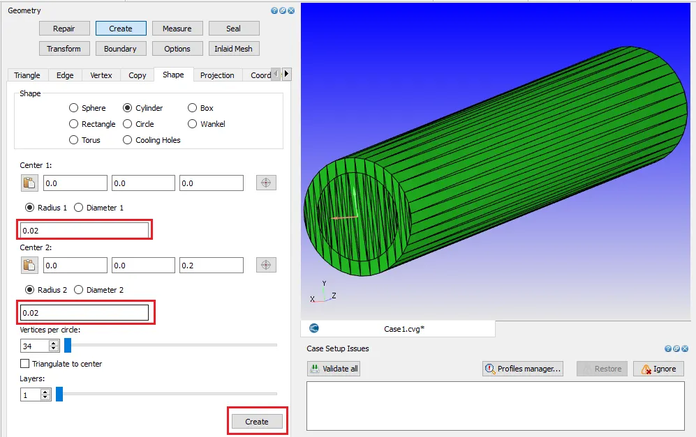
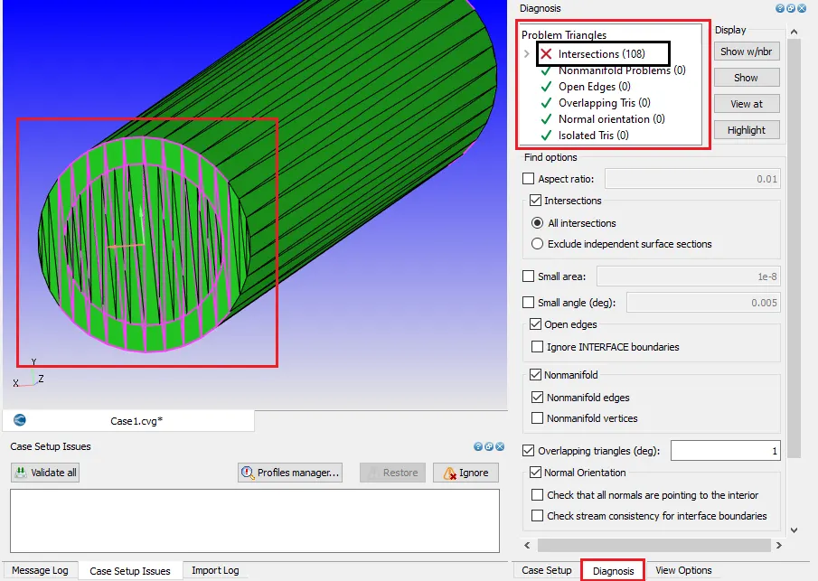
2. Diagnosis:
There is a number of intersections.
3. Removing Intersections:
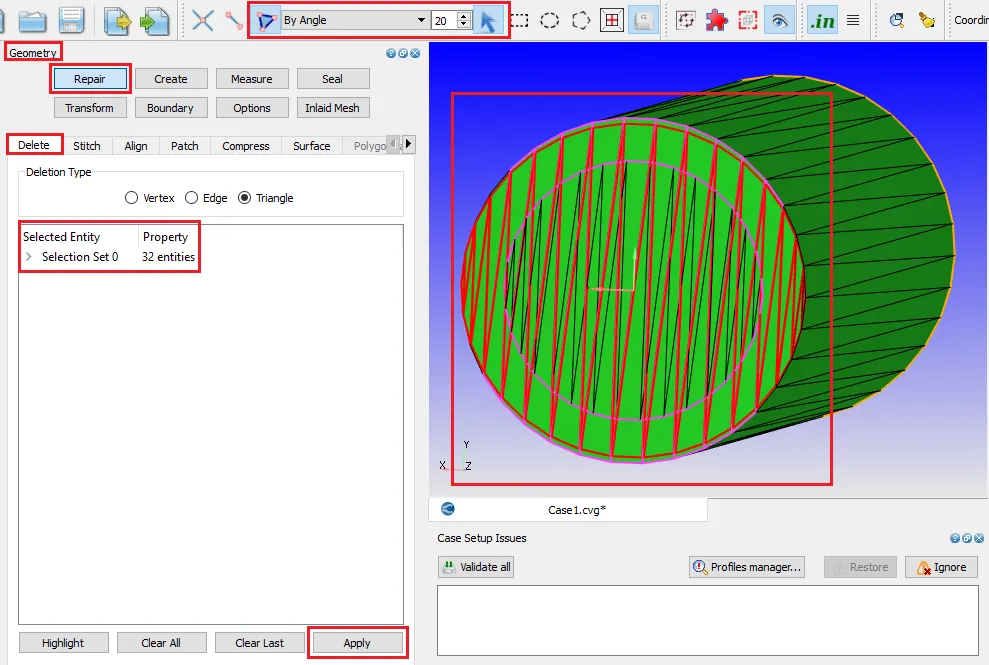
To avoid the intersections in the geometry, deleting the front two faces and back two faces of the geometry.
Repair> Delete> Triangle> `triangle`as an entity> By `20^0` angle> Using cursor pick> Selecting triangles on larger daimeter circular face> Apply
Repair> Delete> Triangle> `triangle`as an entity> By `20^0` angle> Using cursor pick> Selecting triangles on smaller daimeter circular face> Apply
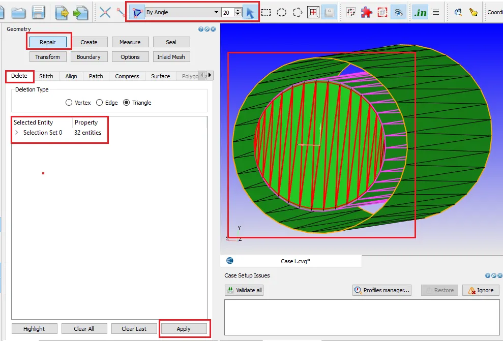
Repeating the same process on the other end of the geometry.
4. Providing Thickness:
To create a flow passage for fluid to separate the fluid body and solid body, providing thickness to the geometry by creating triangles. This will also help in assigning the inlet and outlet boundary.
Create> Triangle - Loft edges> Edge as an entity - By Open Edge> Selecting the larger diameter edge as the first set of edge and then
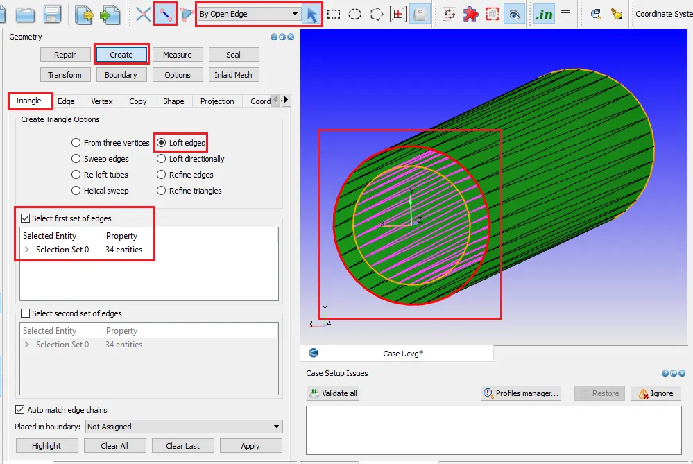
Selecting the smaller diameter as the second set of edge> Apply
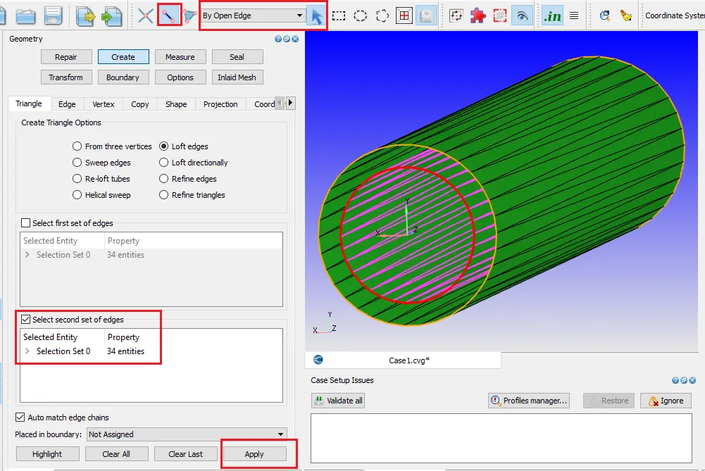
Repeating the same process on the other end of the geometry.
5. Assigning Boundaries:
In converge every part of geometry is assumed to be a triangle. Selecting triangles and grouped to assign to specific boundaries.
Boundary> Flag> +> Create Multiple Boundaries> OK
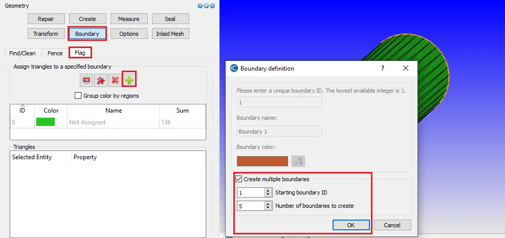
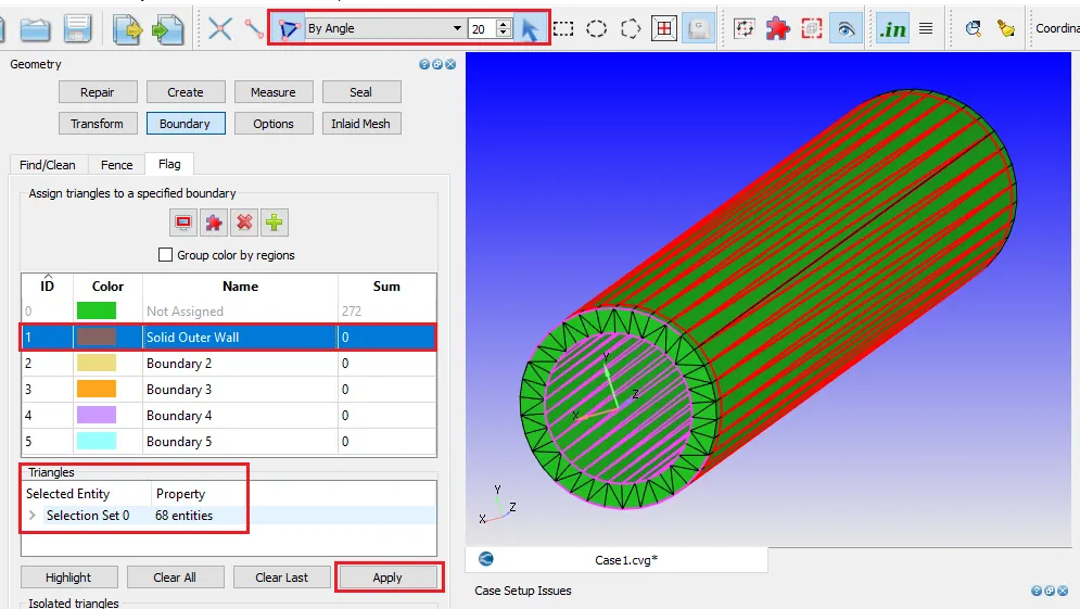
i) Solid Outer Wall:
`triangle` as an entity selection-By Angle `20^0`> Using cursor pick option> Selecting the triangles as shown in below image> Assigning them to Solid Outer Wall Boundary> Apply
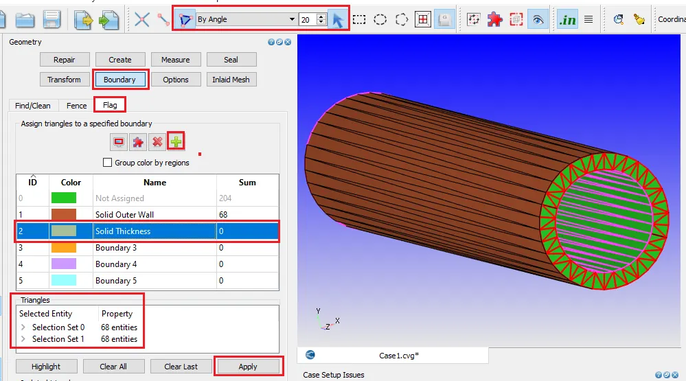
ii) Solid Thickness:
`triangle` as an entity selection-By Angle `20^0`> Using cursor pick option> Selecting the triangles as shown in below image> Assigning them to Solid Outer Wall Boundary> Apply
Similarly, selecting the same triangles on other end assigning the triangles to the same boundary.
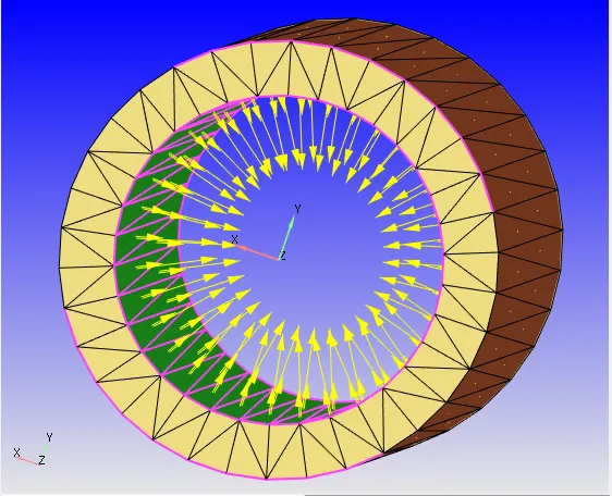
- Normal Orientation: Checking normals before assigning the Inlet and outlet boundaries.
Every geometry has a normal vector, it points perpendicular to it.
Normal Toggle - Enables Normal
To run the CFD simulation, the normal should point towards the fluid.
- Patch: Creating patch on both the ends of the pipe so that the triangles can be assigned to the inlet and outlet boundaries.
Repair> Patch-List of edges> Edge as an entity-By Arc> Selecting inner diameter arc> Apply
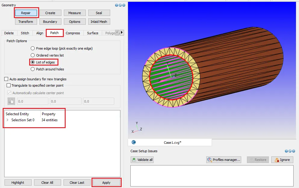
Repeating the same process on the other end of the geometry.
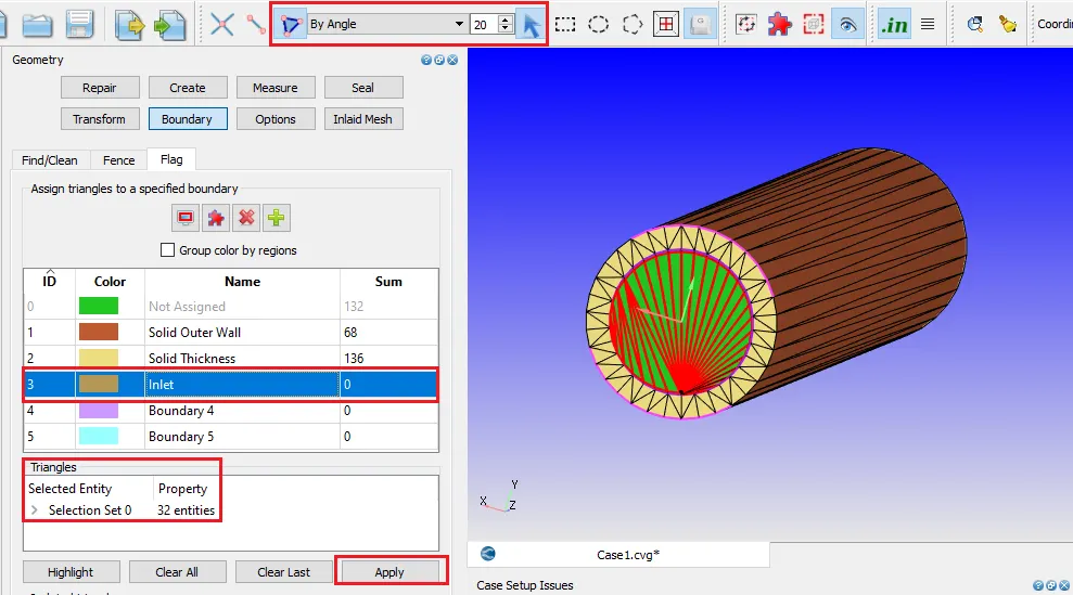
iii) Inlet:
`triangle` as an entity selection-By Angle `20^0`> Using cursor pick option> Selecting the triangles as shown in below image> Assigning them to Inlet Boundary> Apply
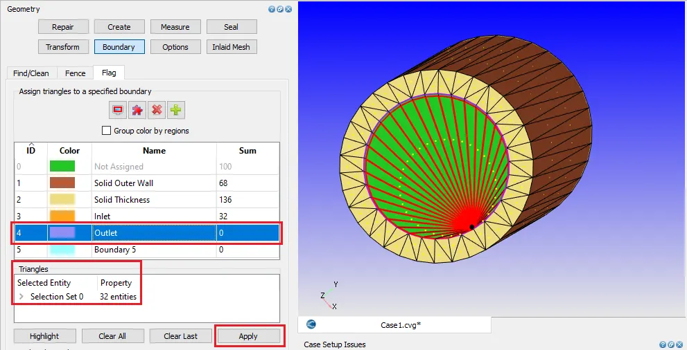
iii) Outlet:
`triangle` as an entity selection-By Angle `20^0`> Using cursor pick option> Selecting the triangles as shown in below image> Assigning them to Outlet
Boundary> Apply
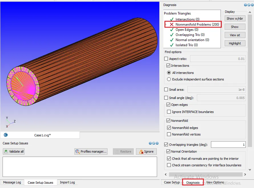
Diagnosis
- Non-Manifold - It can be seen there is a nonmanifold problem, this problem is because of the interface. On one side of the interface, there is solid and fluid on the other side.
- Selecting any one triangle on solid thickness face and hiding the selection.
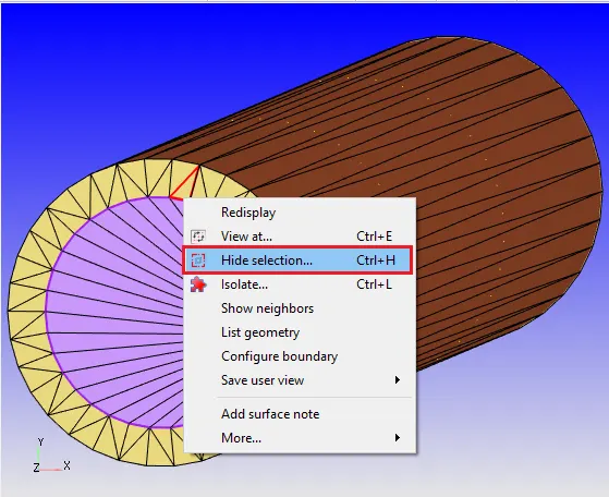
- Selecting the three other triangles, each on the interface, solid thickness and outlet/inlet face. After selecting the triangles isolating them.
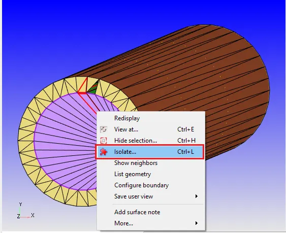
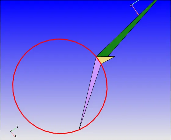
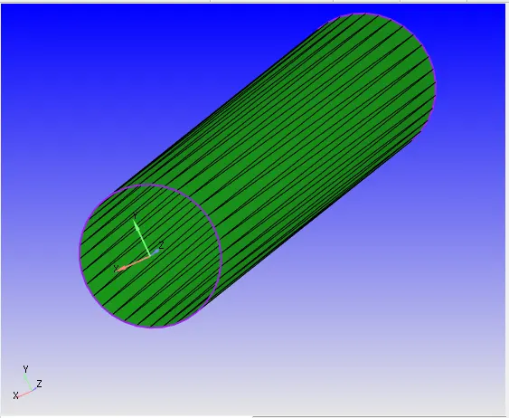
- From the below image it is visible that, edge on the circle is shared by 3 triangles. Similarly, all the edges on the circle are shared by 3 triangles like this. The green triangle is of an interface between solid and fluid, and because of this interface getting non-manifolds.
- Select the triangles as shown below and hide them. After hiding this selection, the only thing will be visible i.e interface.
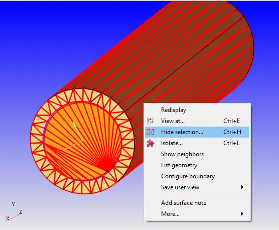
- Interface - This entirely must be assigned to interface boundary.
v) Interface:
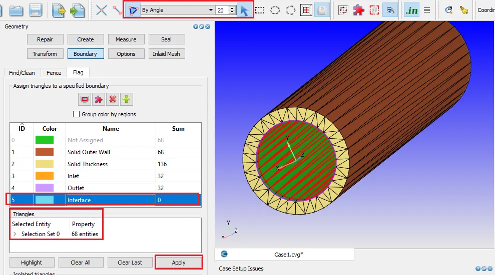
`triangle` as an entity selection-By Angle `20^0`> Using cursor pick option> Selecting the triangles as shown in below image> Assigning them to Interface Boundary> Apply
- Diagnosis:
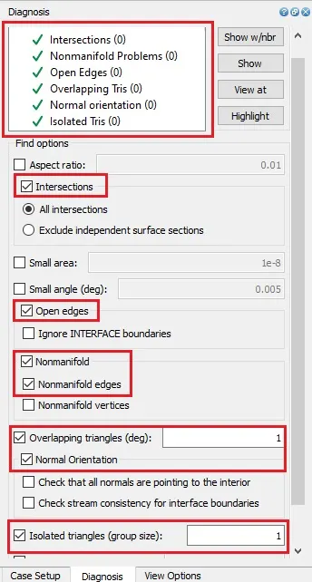
After assigning the triangles to interface boundary, there are no manifold problems present.
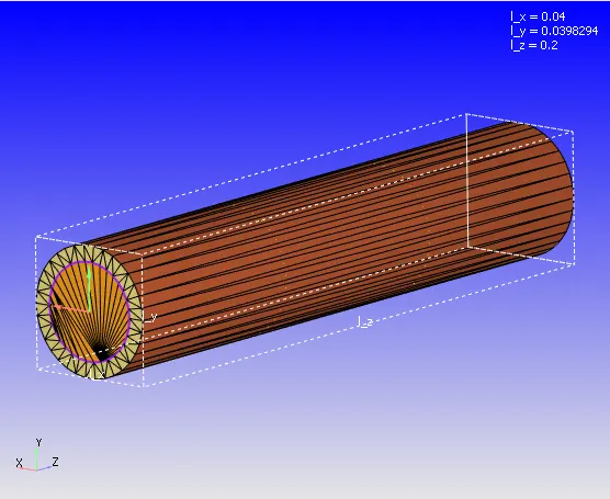
Case Setup:
1. Application Type:
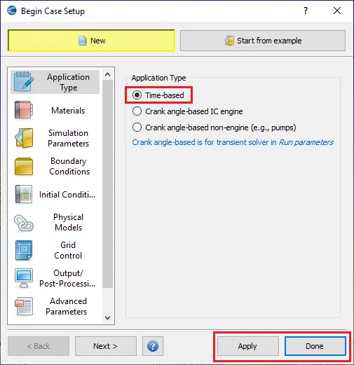
Selecting an application type as "Time Based".
2. Materials:
Gas is flowing through the pipe and the outside is metal.
Checking the solid simulation & Species option and unchecking the reaction mechanism option.
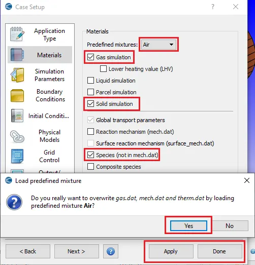
Confirming the permission to overwrite the gas.dat, mech.dat and therm.dat by loading predefined mixture Air.
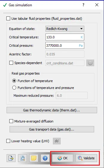
a) Gas Simulation:
Keeping the default values for gas simulation > OK
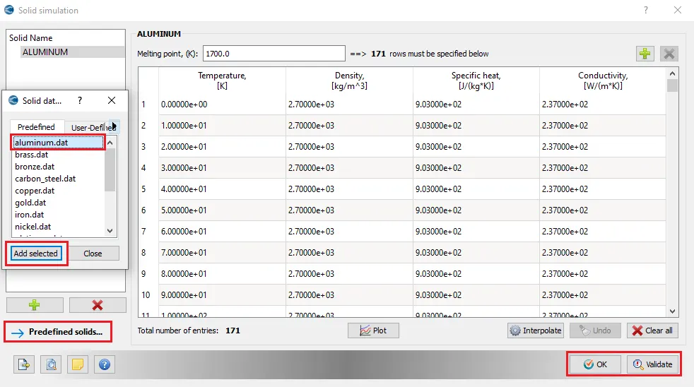
b) Solid Simulation:
Selecting aluminium.dat from predefined solids.
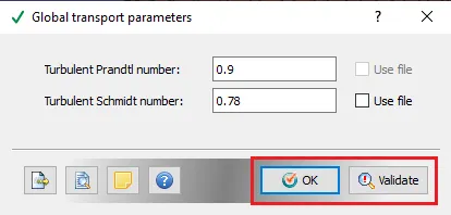
c) Global Transport parameters:
Keeping all the default values for global transport properties > OK
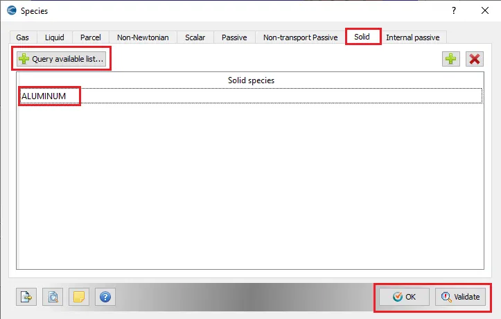
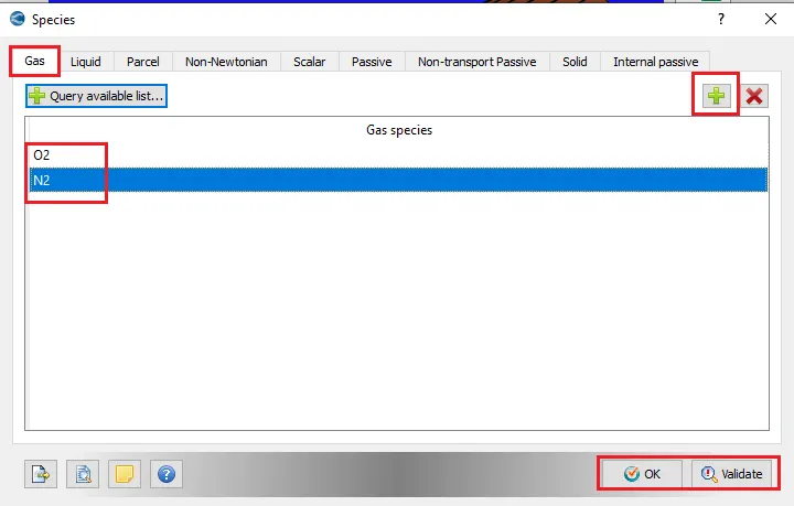
d) Species:
- Solid - From Query available list selecting ALUMINIUM.
- Gas - Adding `N_2` and `O_2`
3. Simulation Parameters:
a) Run Parameters:
Solver: Transient
Simulation mode is Full hydrodynamic and Gas flow solver is Compressible.
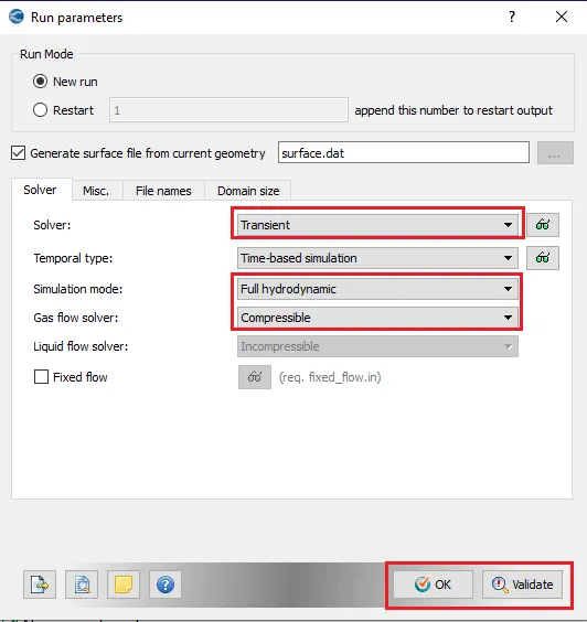
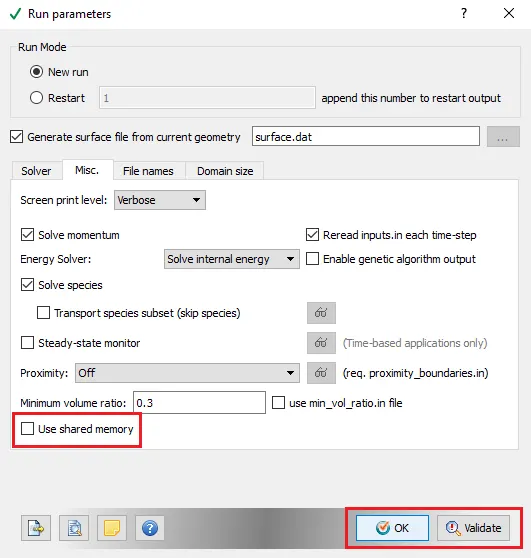
Under Misc. tab disabling use shared memory option > OK.
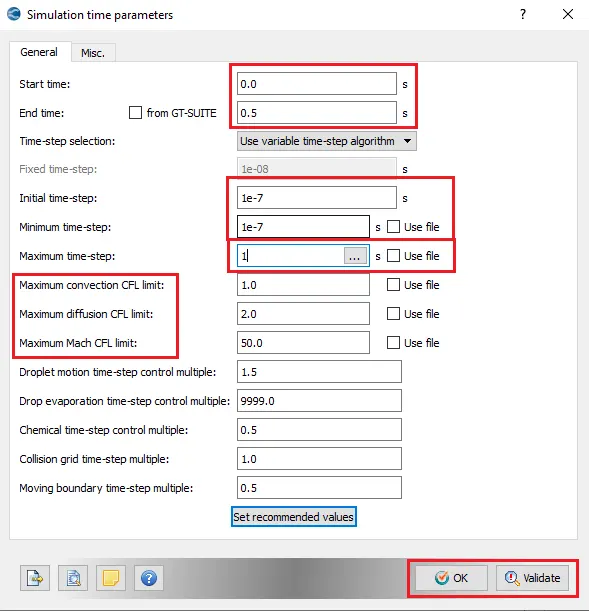
b) Simulation Time Parameters:
Set the start time as 0 s, end time as 0.5 s, Initial and minimum time step as 1e-7 and Maximum time step as 1 second.
Keep all the other CFL values default > OK.
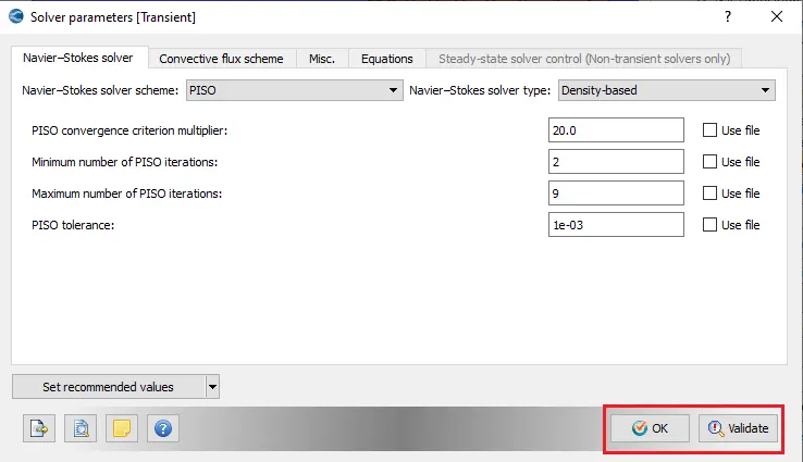
c) Solver parameters:
Keeping all settings as default > OK.
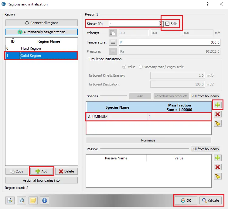
4. Regions and Initialization:
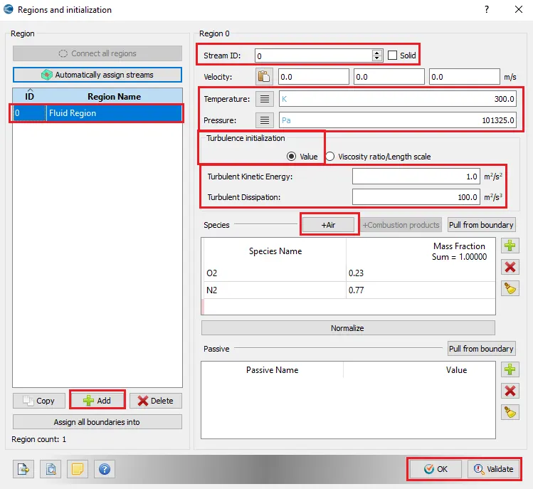
Grouping the boundaries to form volumetric zones called region. This defines a volumetric region with initial conditions like initial pressure, initial temperature, velocity and species concentration
Selecting Add to create a new region,
Add 2 Regions, namely fluid region and solid region.
a) Fluid Region:
For the Fluid Region setting the Stream ID as 0
Velocity - [0, 0, 0] m/s
Temperature as 300 K
Pressure as 101325 Pa.
Select Species as Air
b) Solid Region:
For the Solid Region, setting the Stream ID as 1 and checking the Solid option box.
Temperature as 300K
Species as Aluminium with a mass fraction of 1.00
5. Boundary:
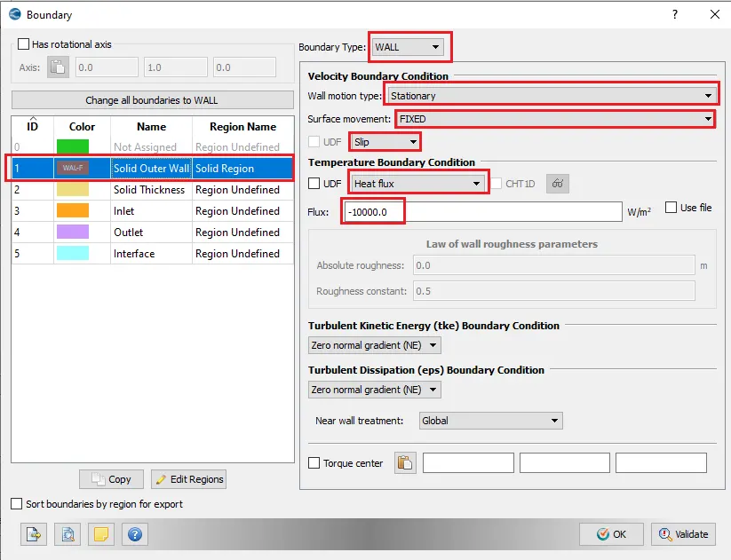
i) Solid Outer Wall:
Boundary Type- WALL
Velocity Boundary Condition:
Wall motion Type - Stationary
Surface Movement: FIXED
Selecting "Slip", Pipe is made up of solid there is no boundary for fluid. The law of the wall is a boundary condition for fluid.
Temperature Boundary Condition:
Selecting "Heat Flux", dealing with conjugate heat transfer problem where the external surface of the pipe is heating with constant heat flux.
Flux: (-10000.0 `W/m^2`) (-ve sign indicates heat is flowing into the system)
Region Name - Solid Region
ii) Solid Thickness:
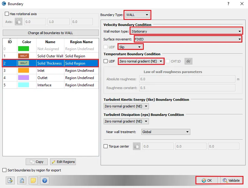
Boundary Type- WALL (Adiabatic Wall)
Velocity Boundary Condition:
Wall motion Type - Stationary
Surface Movement: FIXED
Selecting "Slip", Pipe is made up of solid there is no boundary for fluid. The law of the wall is a boundary condition for fluid.
Temperature Boundary Condition:
Select "Zero normal gradients (NE)" because the wall is adiabatic which means no heat transfer takes place through this boundary.
Region Name - Solid Region
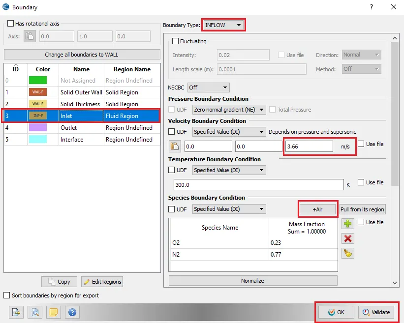
iii) Inlet:
Boundary Type- INFLOW
Pressure Boundary Condition:
Select "Zero normal gradients (NE)"
Temperature Boundary Condition:
Specified Value (DI)- 300K
Velocity Boundary Condition:
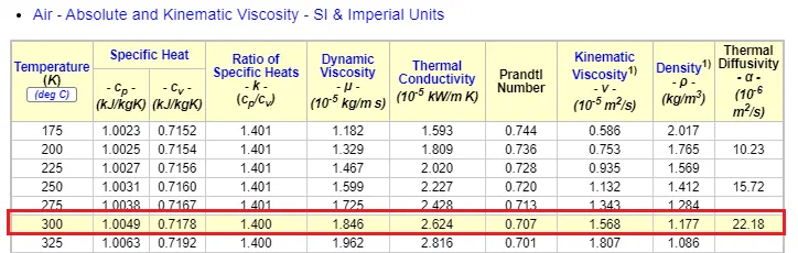
Given: Inlet Reynolds number= 7000
Calculating velocity at Inlet BC based on Reynold's Number
Re = (rho*V*D)/(Dynamic viscosity)
`Re = (rho*V*D)/(mu)`
Where,
Re - Reynolds Number Re = 7000
`rho`- Density of air (@ 300K and 1atm) -`rho = 1.177 (kg)/m^3`
`mu` - Dynamic Viscosity (@ 300K and 1atm) - `mu =0.00001846(kg)/(ms)`
D - Pipe inner diameter - D = 0.03 m
V - Flow velocity
`therefore V=(Re*mu)/(rho*D)`
`V = (7000 times 0.00001846)/(1.177 times 0.03)`
`V = 3.6595 cong 3.66 m/s`
Velocity Boundary Condition:
Specified Value (DI) - `3.66m/s` (in +ve 'z'direction)
Species Boundary Condition: AIR
Region Name - Fluid Region
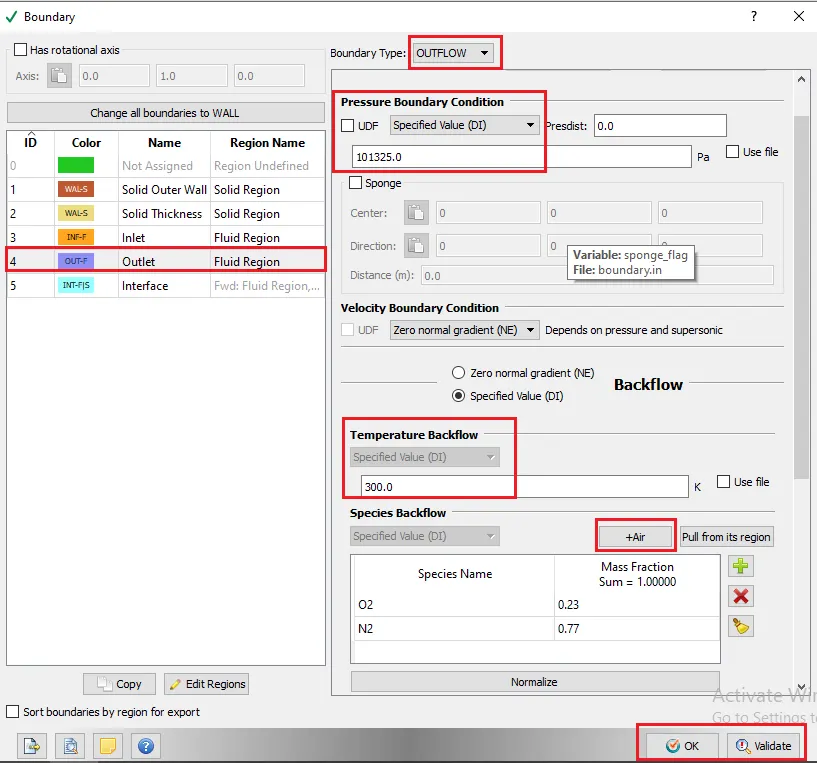
ii) Outlet:
Boundary Type- OUTFLOW
Pressure Boundary Condition:
Specified Value (DI)- 101325 Pa
Temperature Boundary Condition:
Specified Value (DI) - 300K
Velocity Boundary Condition:
Select "Zero normal gradients (NE)"
Species Boundary Condition: AIR
Region Name - Fluid Region
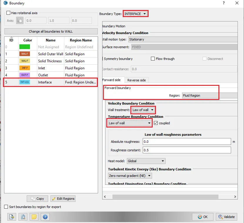
v) Interface:
Boundary Type - INTERFACE
Velocity Boundary Condition:
Wall motion type- Stationary
this boundary is the interface between solid and fluid regions, two different boundaries are set.
a) Forward Side: The boundary which is in the direction of normal of interface boundary called 'FORWARD Boundary'.
Region - Fluid Region
Velocity Boundary Condition - Law of Wall
Temperature Boundary Condition - Law of Wall
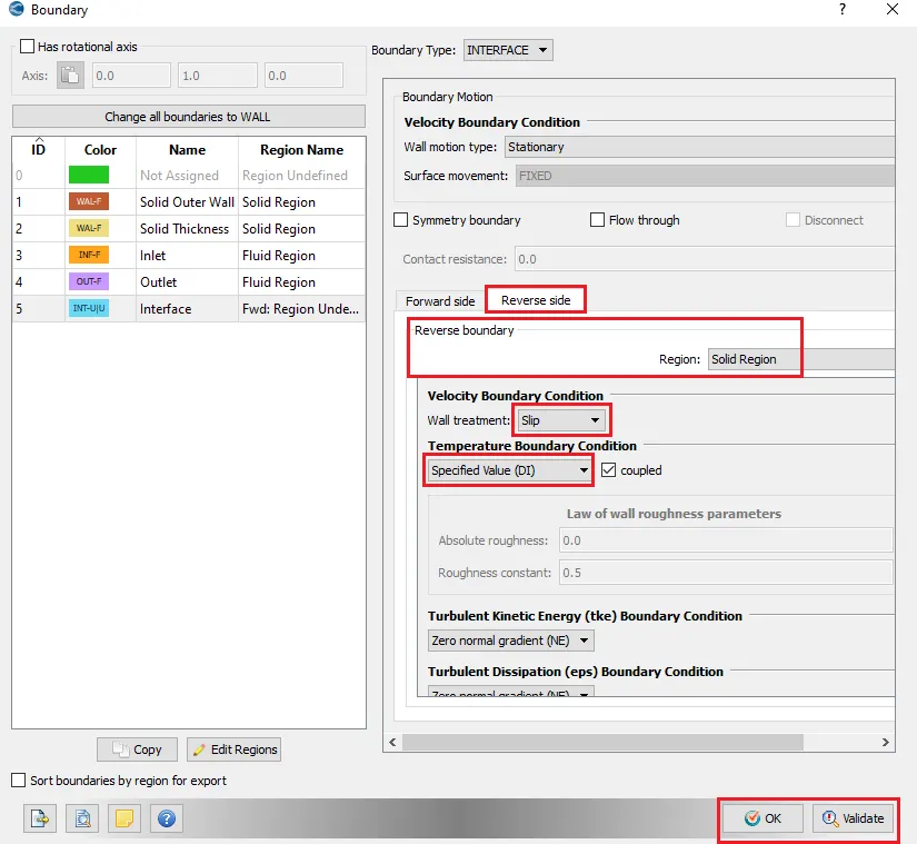
b) Reverse Side: The boundary opposite of normal of interface boundary called 'REVERSE Boundary'.
Region - Solid Region,
Velocity Boundary Condition - Slip
Temperature Boundary Condition - Specified Value
6. Physical:
Enabling Turbulence Modeling
Enabling Super-Cycle Modelling
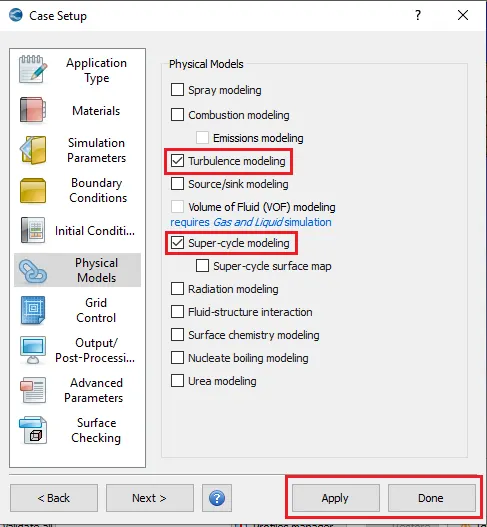
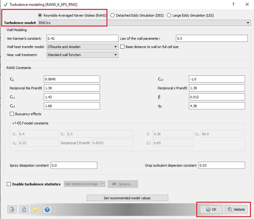
a) Turbulence Modeling:
Keep the Turbulence model as RNG k-epsilon
Keep all the settings default > OK
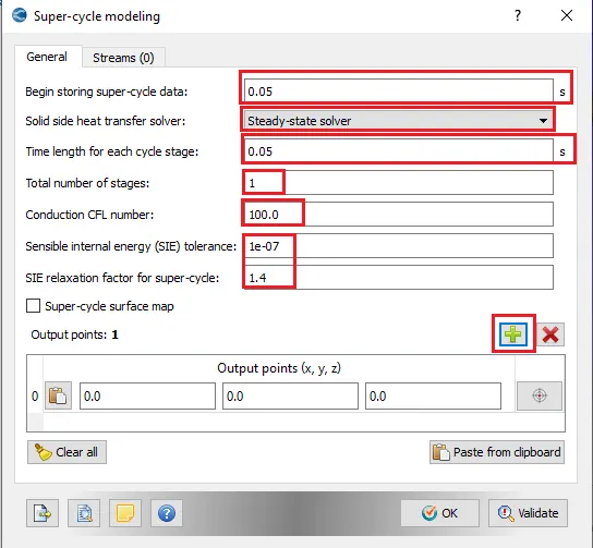
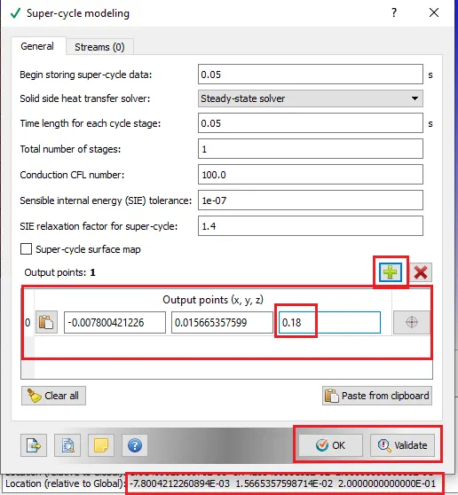
b) Super-Cycle Modelling:
Super-cycling is a method used by CONVERGE Studio in the case of conjugate heat transfer problems with a solid and liquid region.
Solid and fluid, both solvers cannot run at the same speed since solving in the fluid domain is much faster owing to the time scale difference for heat transfer in liquids as compared to solids. This causes problems during the solution given that the solid side solver would not have reached a steady-state/convergence in the time the liquid solver does. This is where the concept of super-cycling can be used.
The basic idea of super-cycling is that the solver for the fluid domain is paused until the solver for the solid domain converges. This pausing is done in intervals that can be set.
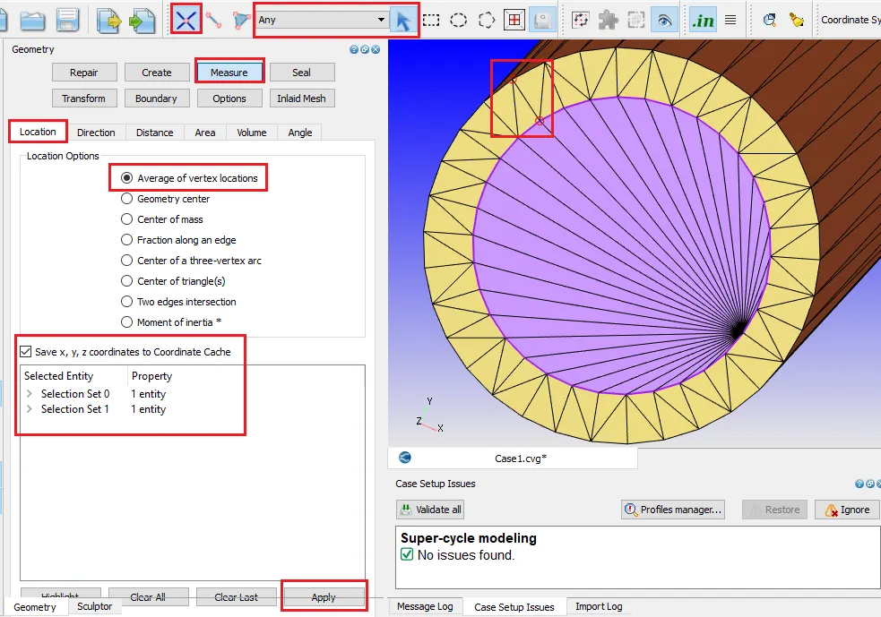
Monitor points: Where temperature to be measured.
Measure> Location-Average of vertex location> Edge as an entity> Using cursor pick option> Selecting 2 vertices> Apply
Pasting the location of monitor points.
Select a point for measuring the temperature convergence near the outlet but little inside the domain.
7. Grid Control:
Kinematic Viscosity - `nu = mu/rho = (0.00001846)/(1.177)`
`nu = 0.000015684 m^2/s`
Skin friction drag coefficient - `C_f =0.0576*Re^(-1/5) = 0.0576 times (7000)^(-1/5)`
`C_f = 0.00980399`
Wall Shear Stress - `tau_w = Cf*(rho*v^2)/2 = 0.00980399 times (1.177 times (3.66)^2)/2`
`tau_w =0.077287898 N/m^2`
Frictional Velocity - `u_t = sqrt(tau_w/rho) = sqrt(0.077287898/1.177)`
`u_t = 0.256310311 m/s`
Assuming the desired y+ = 32
Then first cell centre to boundary distance - `y = y_+ times nu/(u_t) = 32 times 0.000015684/0.256310311`
y = 0.001958126 m
`"Cell Size" = 2 times 0.001958126 times 1000 = 3.9162 mm cong 4mm`
Base Grid:
A grid size of 4 mm.
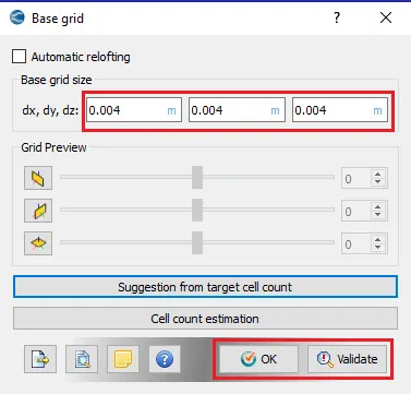
Changing the value of grid size for Grid dependence test.
7. Output/Post-Processing
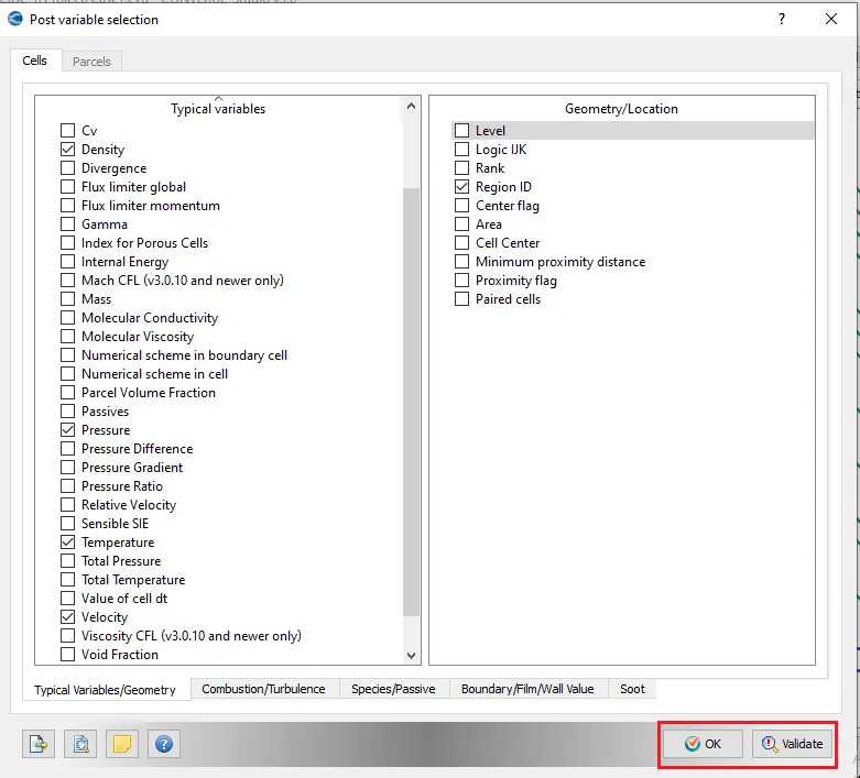
a) Post-Variable Selection
Using default settings for Typical Variables/Geometry.
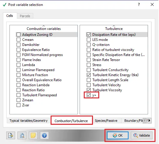
Under Combustion turbulence checking the y+ box in addition to defaults.
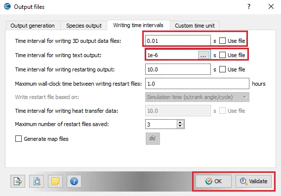
b) Output Files
Setting the time interval for writing 3D output data files - 0.01s
The time interval for writing restarting output to 1e-6
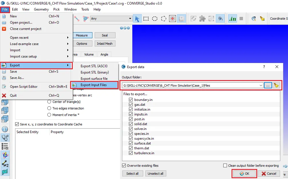
8. Export all the input files
Export all the input files into a separate folder
Files>Export>Export Input Files>setting up the desired location>OK
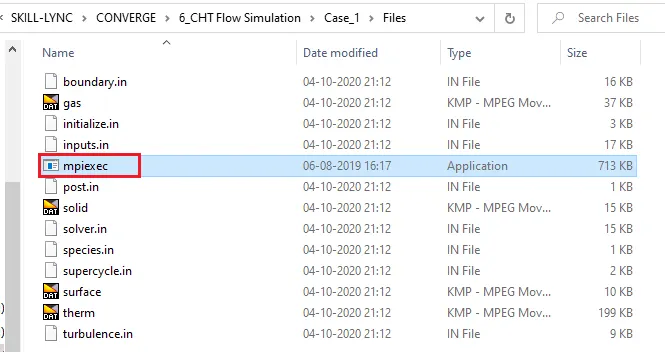
9. Copy and paste the mpiexec.exe file to the input files folder
Run Simulation
Cygwin - Cygwin is a collection of GNU and open-source tools that provide functionality similar to Linux distribution on windows.
To run the simulation, open Cygwin and navigate to the folder in which the input files are exported.
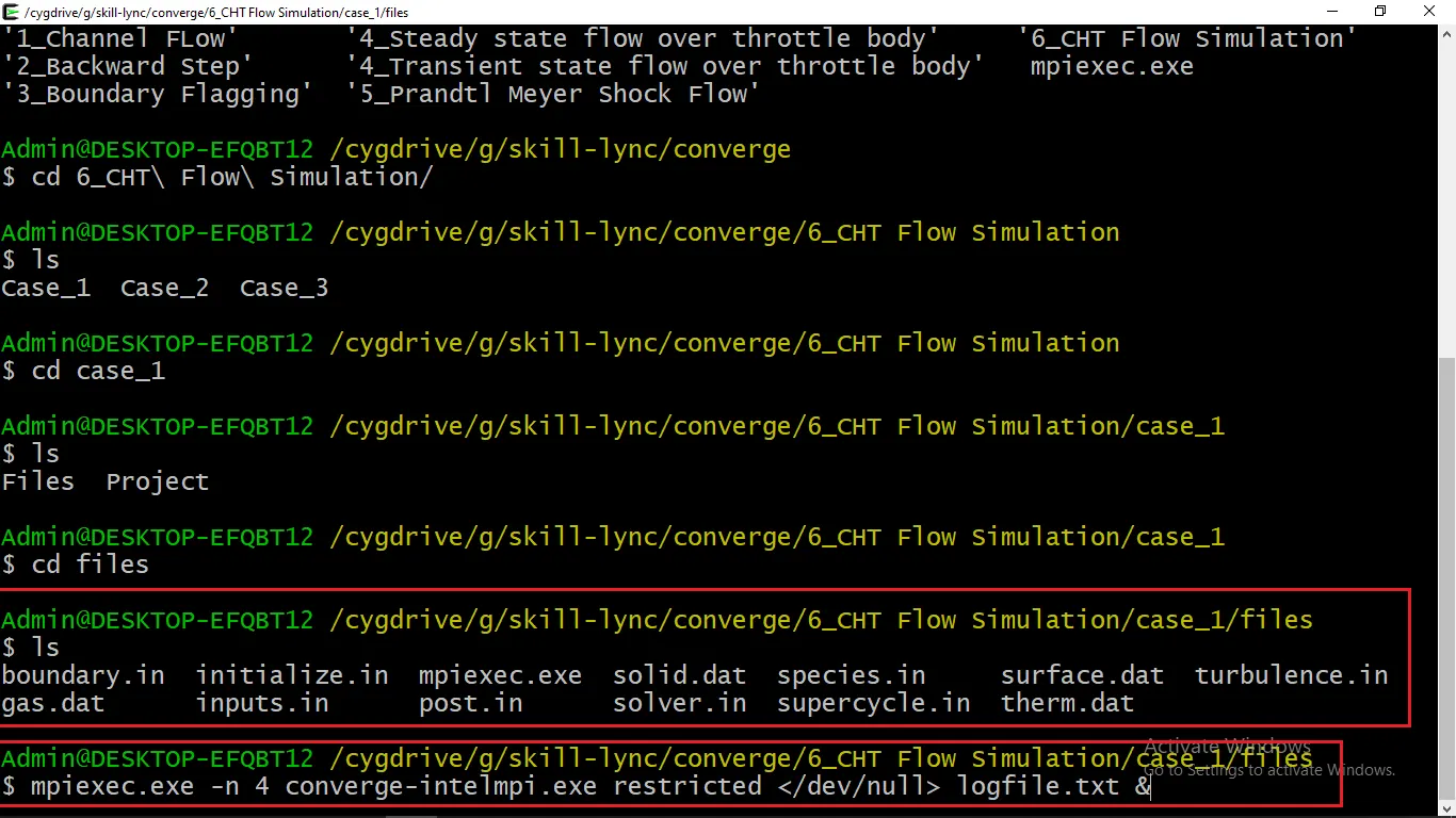
To run the simulation command with executable to be entered
$ mpiexec.exe -n 4 converge-intelmpi.exe restricted logfile.txt &
Taking output mpiexec.exe and sending it to further Taking data from and sending to logfile.txt
Grid Dependence Test:
- Starting with an initial base grid of 4mm grid size running grid dependence test on 3 grids.
Case 1 - 0.004m grid size
Case 1 - 0.003m grid size
Case 1 - 0.002m grid size
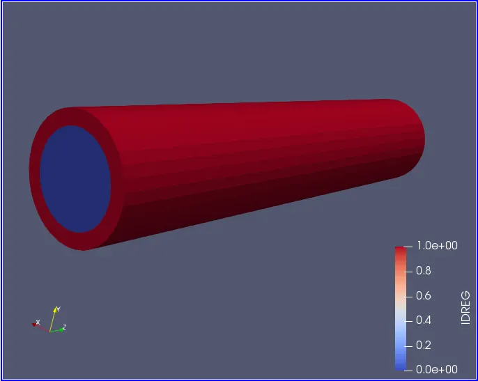
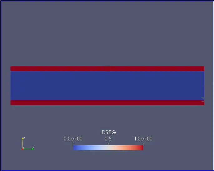
Geometry with region representation:
Grid Dependence Test:
Results:
Case 1 - 0.004m grid size
Case 1 - 0.003m grid size
Case 1 - 0.002m grid size
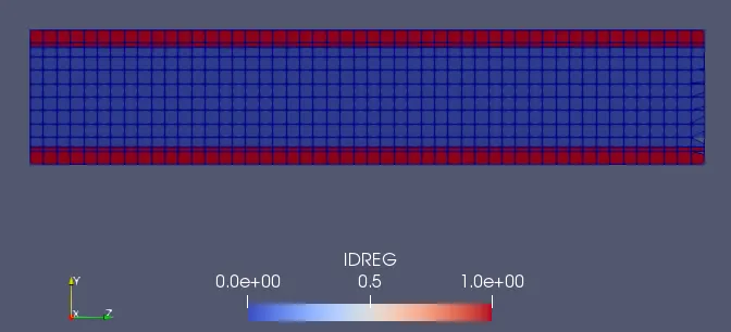
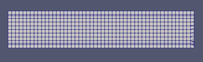
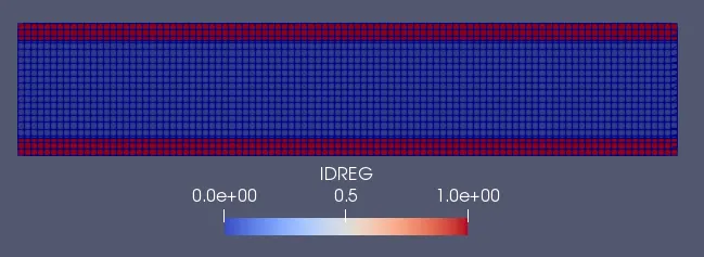
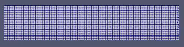
Meshing:
Case 1:
Case 2:
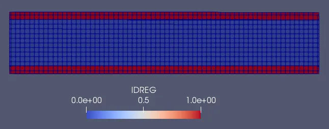
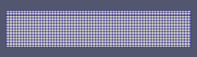
Case:3
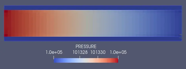
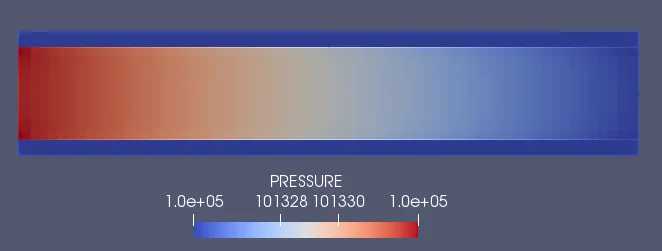
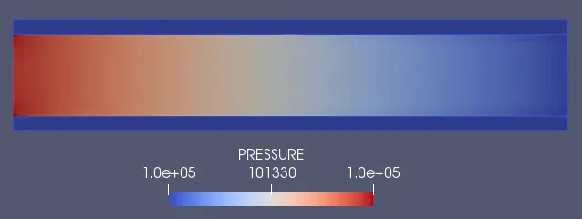
Pressure Contour:
Case 1:
Case 2:
Case 3:
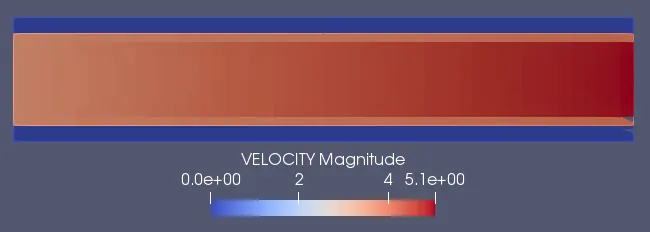
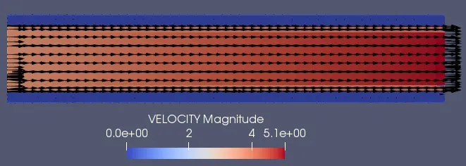
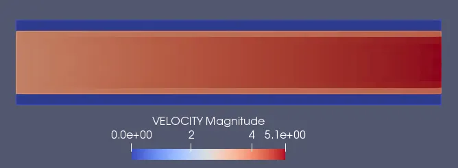
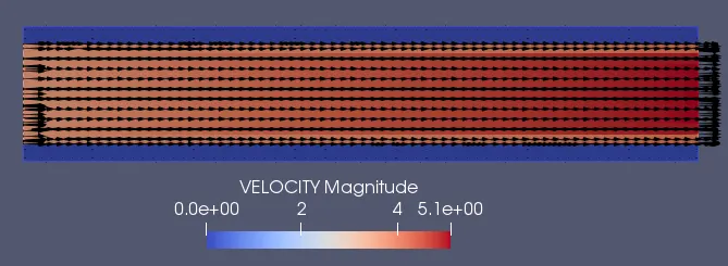
Velocity Contour and Vector representation:
Case 1:
Case 2:
Case 3:
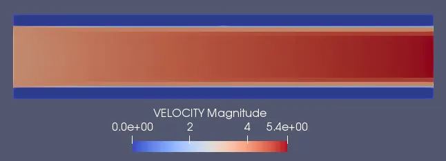
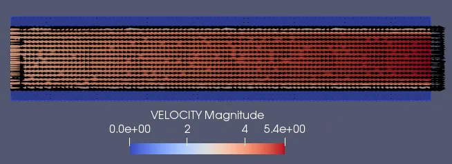
The using finer mesh has given precise details of changes in flow pattern in earlier problems. Similarly, in this case, also it can be observed that as mesh size is reduced to 0.002m finer flow contour of temperature, velocity and y+ boundary value are obtained.
Temperature Contour:
Case 1:
Animation:
Case 2:
Animation:
Case 3:
Animation:
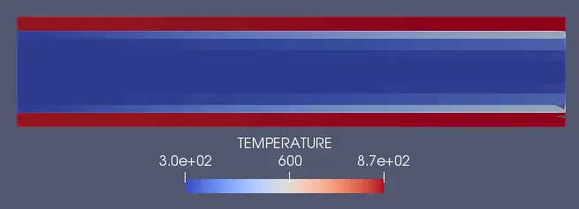
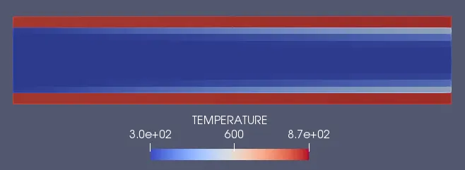
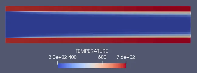
From the above temperature contour for all 3 grids, if observed near the outlet side there are clear differences in all 3 grids. With more refinement, the outlet temperature has converged to slightly different Values. Even the coloured profile observed in the base grid just below the solid region is less dense but as moved to grid 0.003m its more shaper and even more at the final grid 0.002m.
y+ Contour:
Case 1:
Case 2:
Case 3:
Animation:
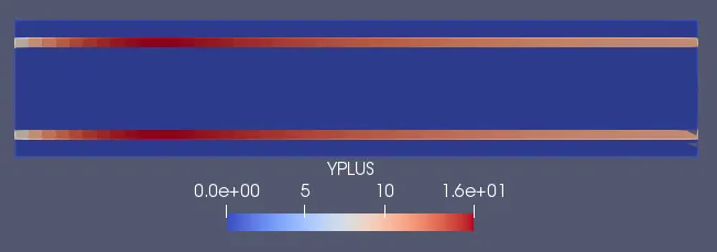
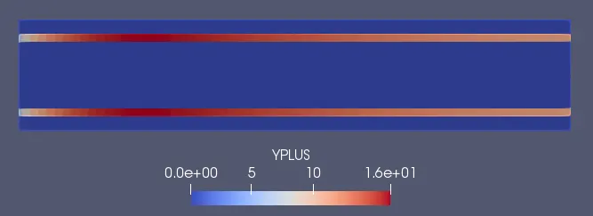
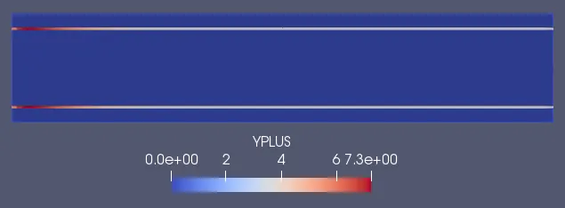
Near-wall regions have larger gradients in the solution variables, and momentum and other scalar transports occur most vigorously. The wall y+ is a non-dimensional distance similar to local Reynolds number, often used in CFD to describe how coarse or fine a mesh is for a particular flow. It is the ratio between the turbulent and laminar influences in a cell.
Accurate presentation of the flow in the near-wall region determines the successful prediction of wall-bounded turbulent flows. Values of y+ close to the lower bound (y+≈30) are most
desirable for wall functions whereas y+≈1 are most desirable for near-wall modelling.
However, we have a problem when the y+ lies in the range between 10 and 30. Here, it is not easy to predict the solution in the transition region. The best practice here is to go finer to the laminar region and just use the no-slip condition or another idea would be to use a coarser grid and go for a wall function instead.
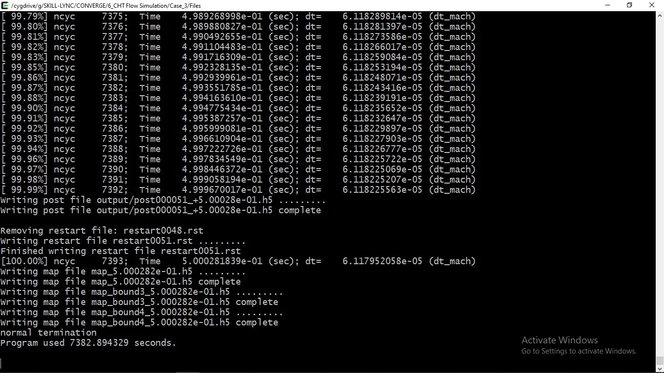
Computational Time:
Case 1:
Case 2:
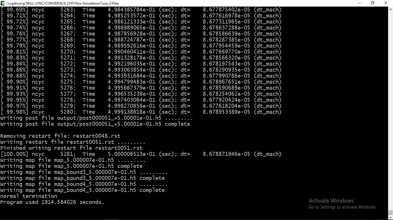
Case 3:
Temperature Plots:
i) FLuid Region:
ii) Solid Region:
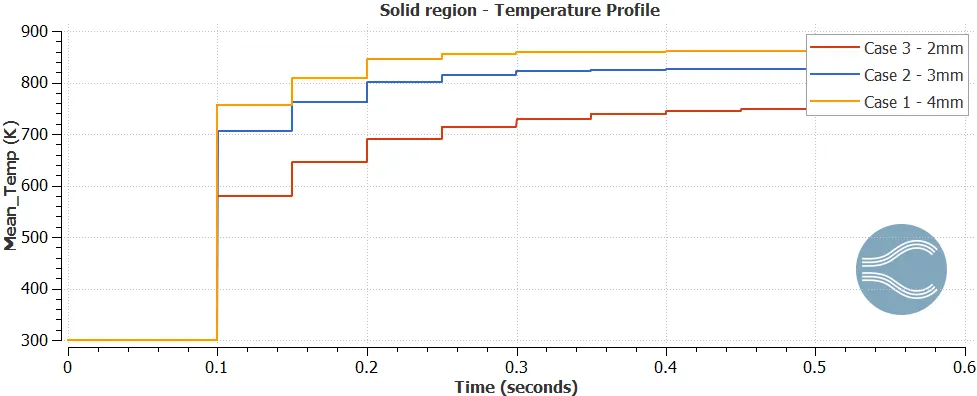
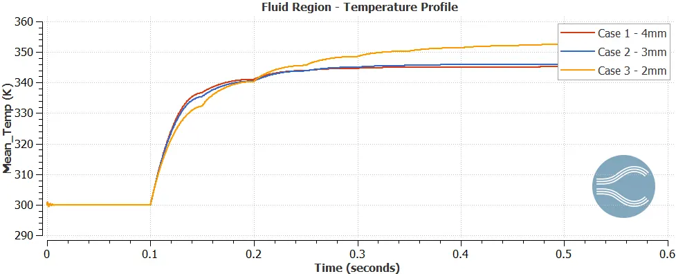
The above plots show the mean outlet fluid temperature and solid temperature for three different grid size values. Although they do not converge to the same specific value, they all are around a decent margin. It is clear that the fluid temperature is going to be around 350 K and the solid temperature around 850 K. It can also be seen that the temperature change is quite significant and is grid-dependent.
Choosing more finer mesh would provide us with some reliable results but with a current computational resource mesh size of 0.002m is more reliable and can be concluded that mesh size smaller than 2mm can show a grid-independent nature.
It can be also observed that coarser mesh converges at a faster rate but a finer mesh provides accurate results. We can see that for finer mesh the solid region mean temperature is low, whereas the liquid region means the temperature is high for a finer mesh. Here the temperatures are sensitive to changes in mesh grids and hence we can reduce the mesh size further to obtain high-level accuracy until these results become independent of the mesh.
Effect of supercycle stage interval:
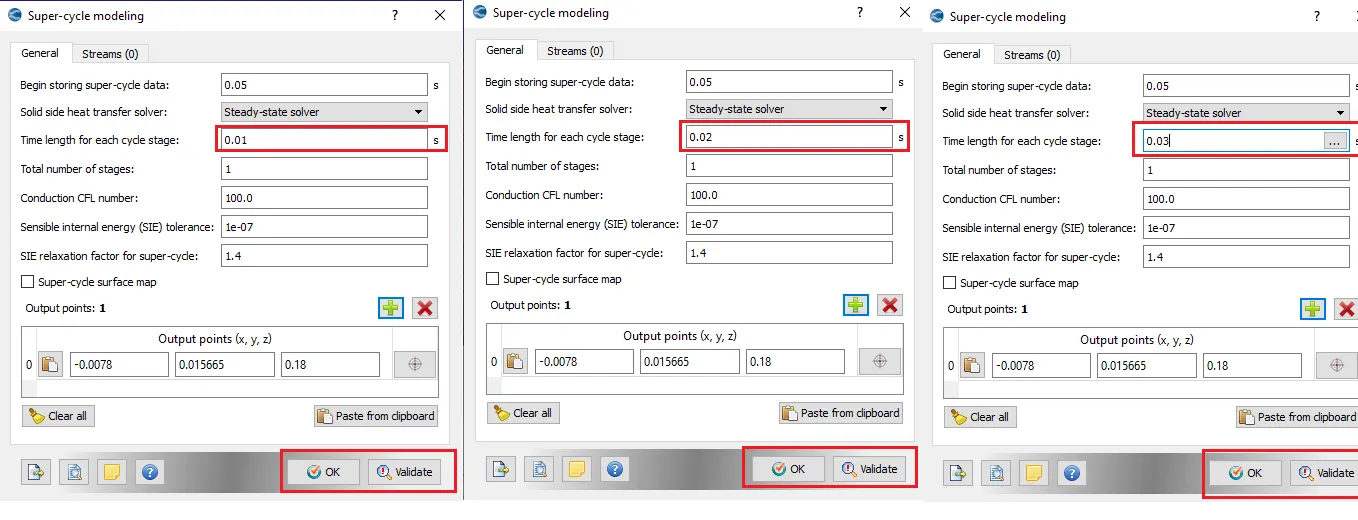
- Setting the supercycle stage interval to 0.01,0.02 and 0.03
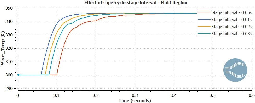
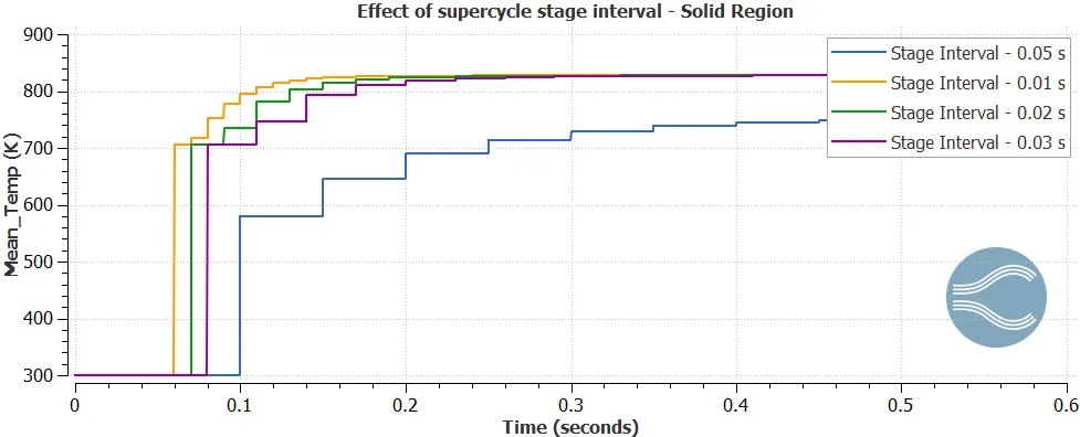
The mesh grid size is 0.003m and different supercycle stage interval values of 0.05s (baseline configuration), 0.03s, 0.02s & 0.01s are compared.
i) Fluid Region at Mesh size = 0.003m at Supercycle stage interval of 0.05s, 0.03s, 0.02s & 0.01s
Supercycle temperature plot Fluid region:
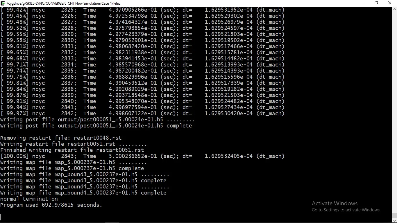
From processing the files in Cygwin it was observed that as supercycle values are reduced higher the time is taken for processing it (i.e. comparison to baseline configuration of 0.05s with 0.03s, 0.02s & 0.01s). The above temperature curve attains convergence early at the lowest value of supercycle amongst the values given. This could be employed for finer mesh where convergence delays to attain it at a faster rate. Hence, thereby the end time could be shortened which could save the solving time.
ii) Solid Region at Mesh size = 0.003m at Supercycle of 0.05s, 0.03s, 0.02s & 0.01s
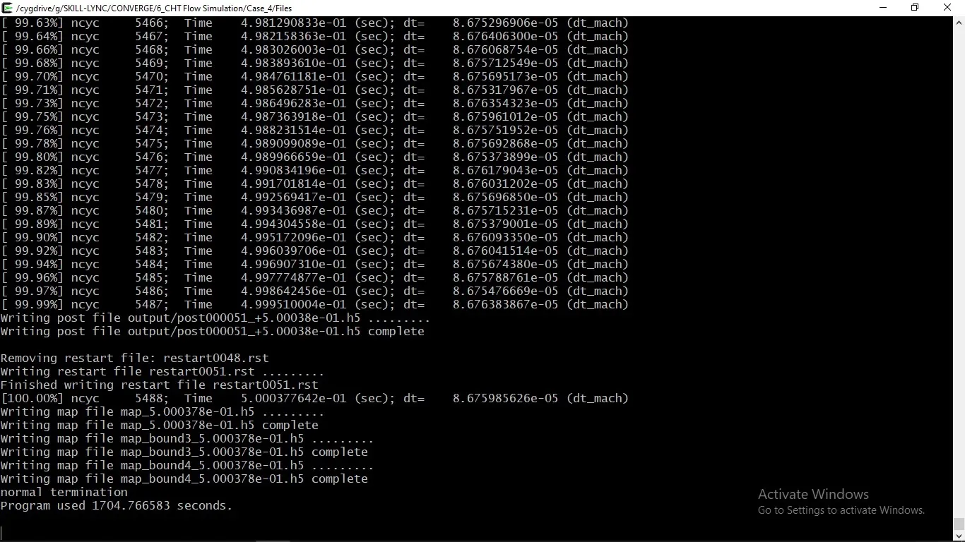
Computational Time for Different Super Cycle stage intervals:
Case 1:
Time length for each cycle stage=0.01
Case 2:
Time length for each cycle stage=0.02
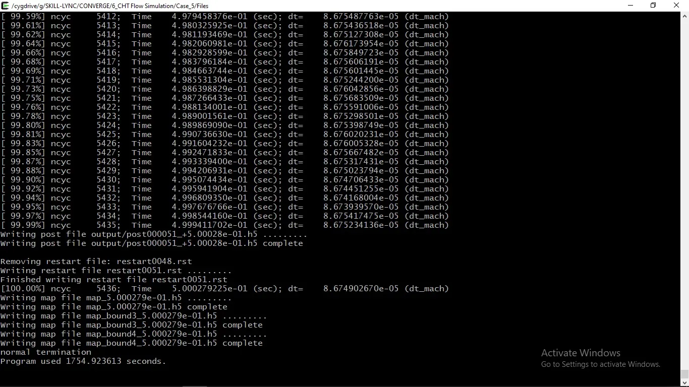
Case 3:
Time length for each cycle stage=0.03
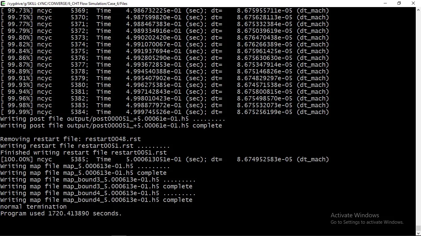
No major difference is observed in simulation time and mesh size considered here is 0.003m for all supercycle stage interval. Simulation time is only affected when the grid size of the geometry is changed.
Y+ Data:
1. Y+ is a non-dimensional length scale that is normalized using wall shear stress. Since each turbulence model simulates the boundary condition, so the value of Y+ is an important parameter to predict the flow field of the boundary layer. The turbulent boundary layer consists of 3 layers (Viscous sub-layer, logarithmic region and the Buffer layer) wherein different relations are observed between the average velocity and this non-dimensional distance y+.
Max y+ value for different mesh Size according to the case:
1. 0.004m 16
2. 0.003m 16
3. 0.002m 7.3
The above values of y+ in different mesh grids are independent of supercycle values at the mesh size.
Below picture assigns regions to different values of y+.
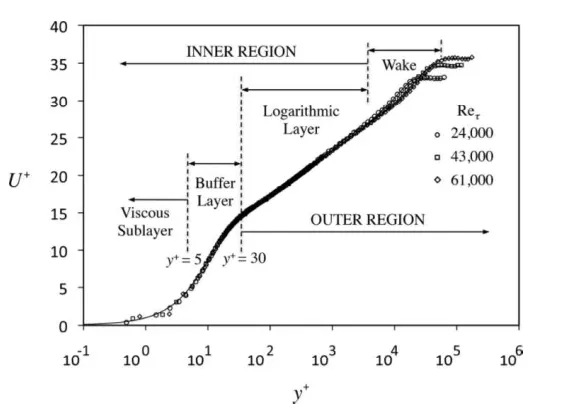
a. The viscous sublayer lies for y+ <=5.
b. The buffer layer lies in 5<y+<30
c. The logarithmic layer y+ = 30-100, up to 500.
Hence we can say that for this simulation the flow regime lies in the buffer layer.
2. The difference between the time scales of the solid region and the fluid region is overcome by super-cycling with the basic idea that the solver for the fluid domain is paused (done in intervals) until the solver for the solid domain converges. The effect of super-cycle can be observed that at lower super-cycle stage interval values the flow converges early (i.e. comparison to baseline configuration of 0.05s with 0.03s, 0.02s & 0.01s) which can be employed to solving finer mesh for reducing solver time by reducing end time in seconds. Super-cycling significantly reduces the computational cost of the CHT simulation.
3. From the grid dependency test it can be concluded that as the mesh size reduces y+ value reduces. Moreover, it is found that the value of mean temperature varies as the mesh size changes and mesh size can be reduced to increase accuracy until the flow contours become independent of it. Hence, further the size of the mesh can be reduced until the percent changes in sequel mesh grids are negligible.