Conjugate Heat Transfer Simulation

Conjugate Heat Transfer Simulation

Aim: To perform a Conjugate Heat Transfer flow simulation through a pipe in Converge CFD and post processing the results.

Objective:

• To setup flow simulation though a pipe.
• Considering the Reynolds as 7000 and calculating the velocity alue by using

Re = (rho*V*D)/(Dynamic viscosity)

• To perform a grid dependence test and show that the outlet temperature converges.
• To run the simulation by varying the grid sizes and by changing the supercycle stage interval(0.01,0.02,0.03) and comparing them to the baseline configuration.

Description:

The exchange of thermal energy between the two physical bodies is called as the study of heat transfer. The rate of transferred heat is directy proportional to temperature difference between the bodies.Conjugate Heat Transfer is a process which involves variations of temperature within solids and fluids, due to thermal interaction between the solids and fluids. WHen we have multiple modes of heat transfer i.e. conduction /convection it is called as CHT. Wall functions are generally used o calculate the solution near the wall. Y+ is a dimensionaless quantity that can be used to understand the kind of mesh. This is used to determine if the wall functions need to be used or not. The Turbulent flow have a smaller laminar region near the wall.

Super cycling is a method that is used in converge to solve CHT simulations/problems. Converge solver solves the solid region and fluid region seperately. The time scale difference between both the regions is very high. This is because time required for solver to attain steady state in fluid region is very small when compared to that of solid. In supercycling, the solver is paused in the fluid domain untill the solid domain reaches steady state. This pausing is called as supercycling stage interval and this is set manually as per our requirement.In Converge, fluid heat transfer uses the Navier stokes equation and solid heat transfer uses energy equation.

3D-Tranient heat conduction equation

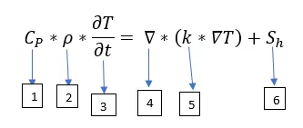
Where,

1- Specific Heat 2- Density 3- Rate of change of temperature w.r.to time

4-Divergence 5- Conductivity 6- Volumetric Heat source

To solve the equations we need boundary conditions.These Bc are provided most slightly between the solid and the fluid where the fluxesfrom fluid directly match the fluxeson the solid side.In order to understandthe temperature distribution in solid component we need to perform Heat transfer simulation. If the heat is transfered to solid through some type of gas phase or liquid phasemedium, then we need to do CHT.

Procedure:

• Initially open Converge Studio and create the geometry i.e. creating a fluid region and solid region. By specifing the radius values create a two cylinders in order to form solid region and fluid region.

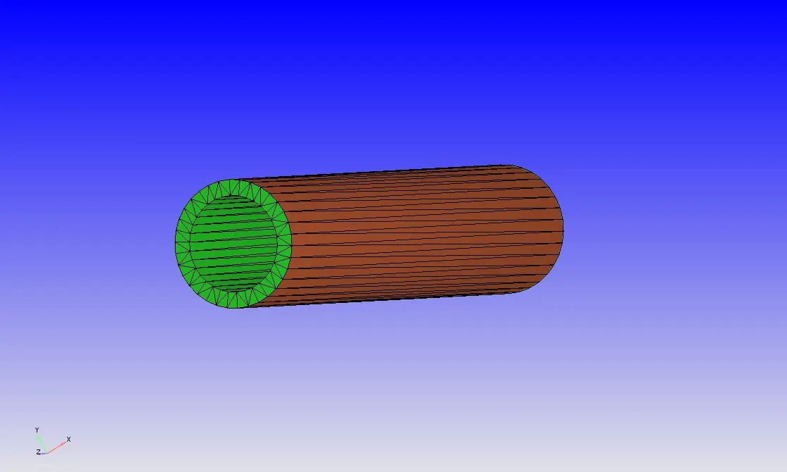
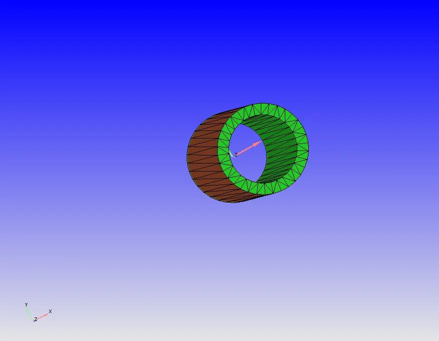
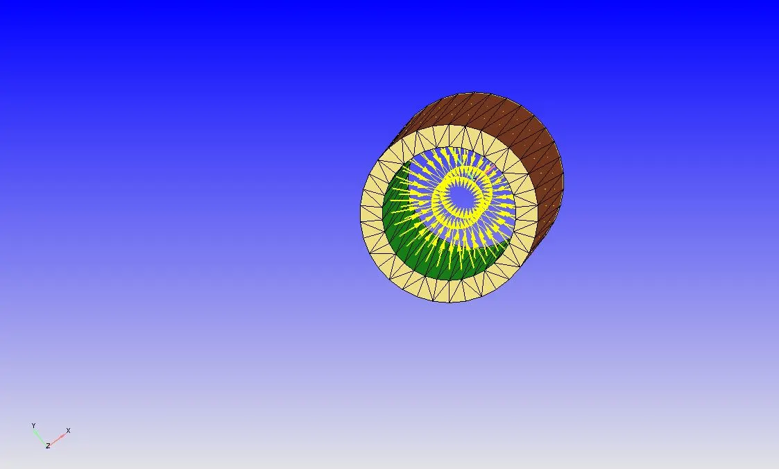
• Delete the intersections from both the regions. Next to form regions use loft option.Now identify the inlet and outlet and patch them.

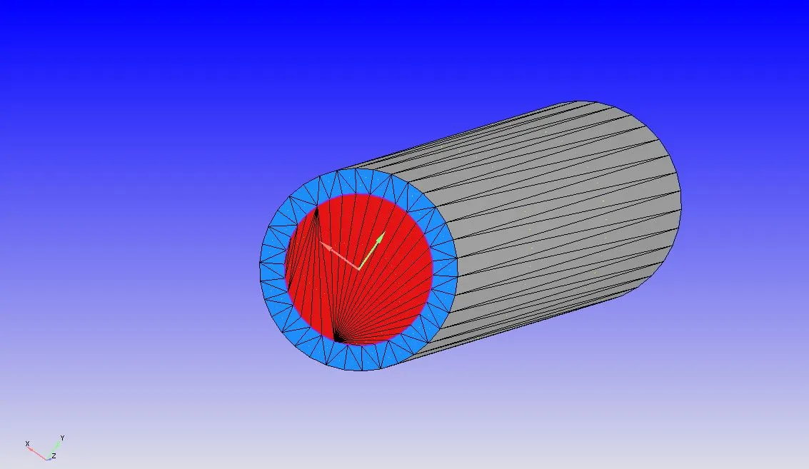
• After setting the geometry, next important thing is to diagnosis the geometry for errors/problems. For this go to Right Bottom side, select Diagnosis > click on All intersections > click Find. On top we can check for problems in Problem Triangles.
• Now if there are no errors found then the geometry is correct.
• To we should do Case Setup. Just beside Diagonisis > click on Cae Setup > in case setup window we can see 'Begin Case Setup" > click on it to set the setup.

Case Setup-

Application Type = Time-based

Materials -

Predefined mixtures = Air

Select 'Gas Simulation', 'Solid simulation' and 'species'.

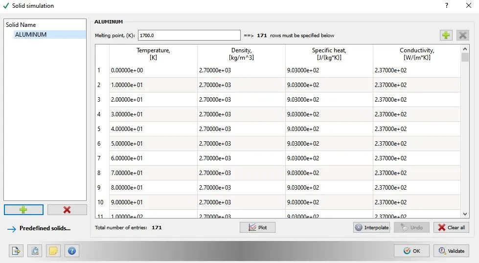
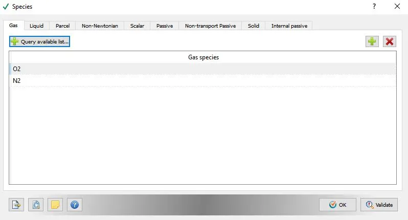
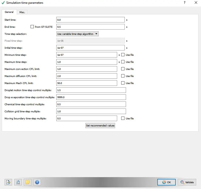
Simulation Parameters-

In Run Parameters two main things to be considered:-

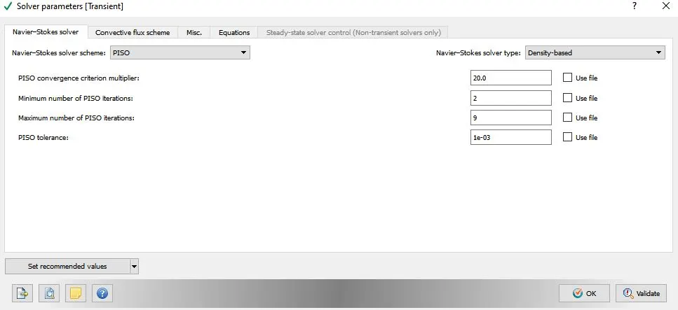
(a.) select the following solver settings

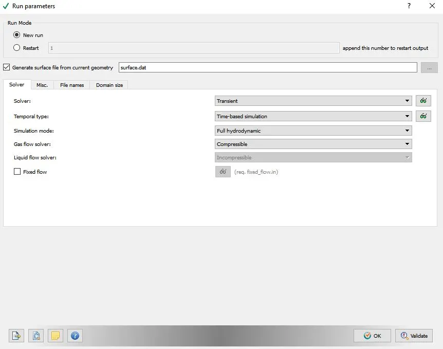
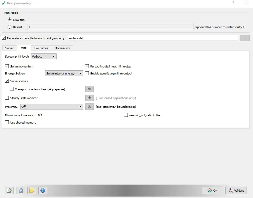
Simulation Time Parameters-

Solver Parameters [Transient]-

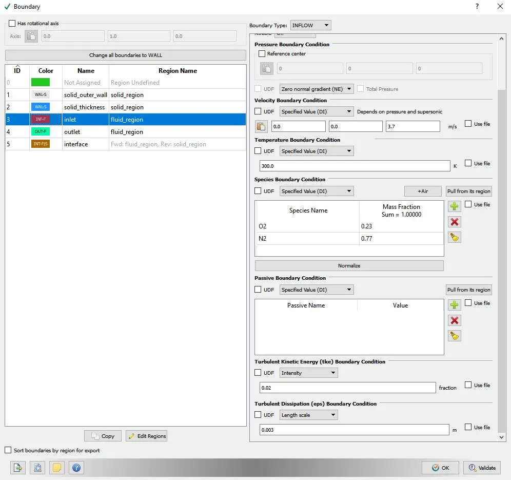
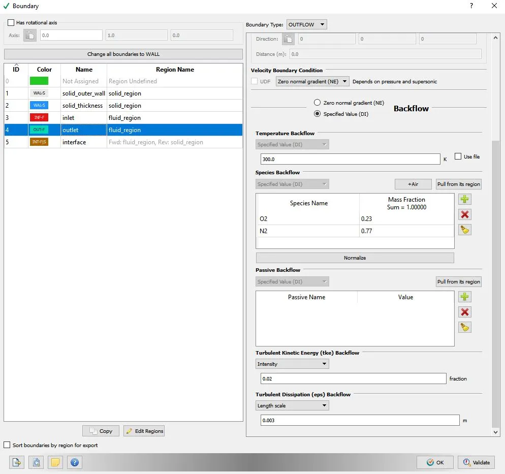
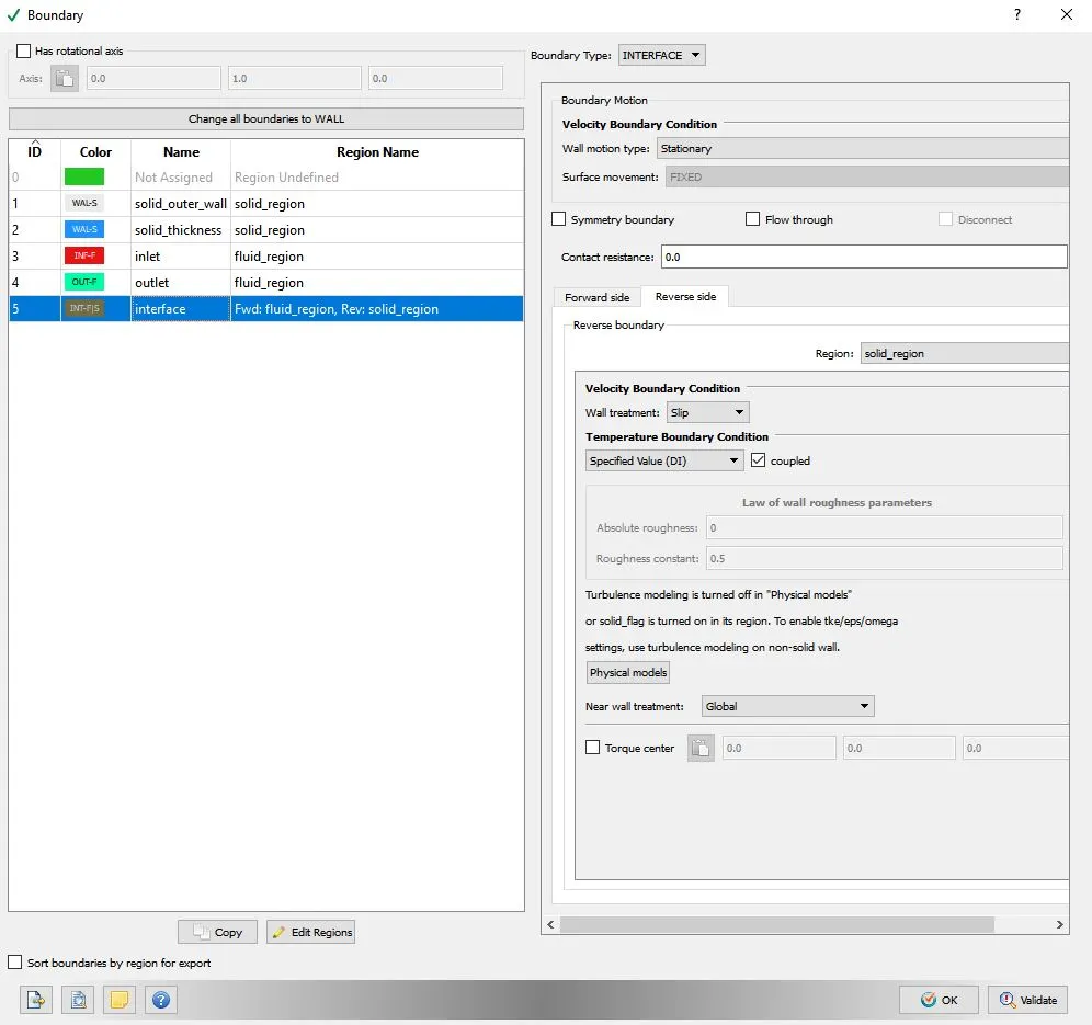
Boundary Conditions-

Boundary:

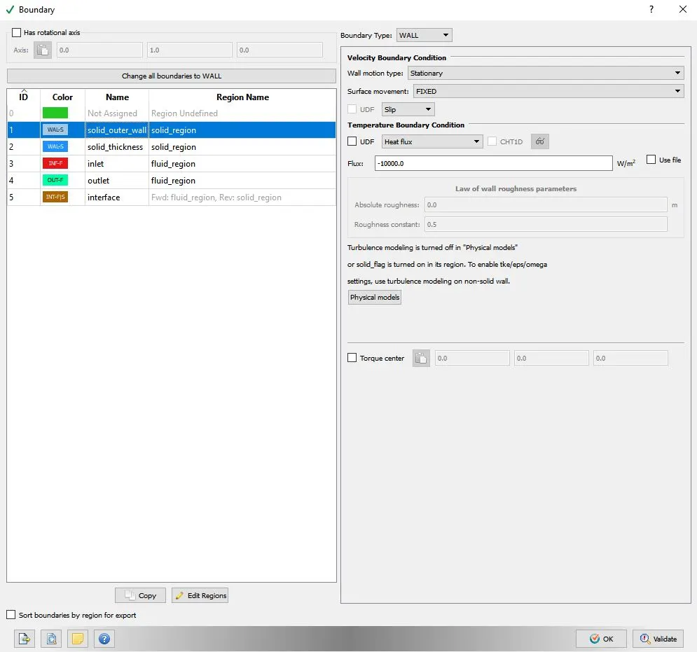
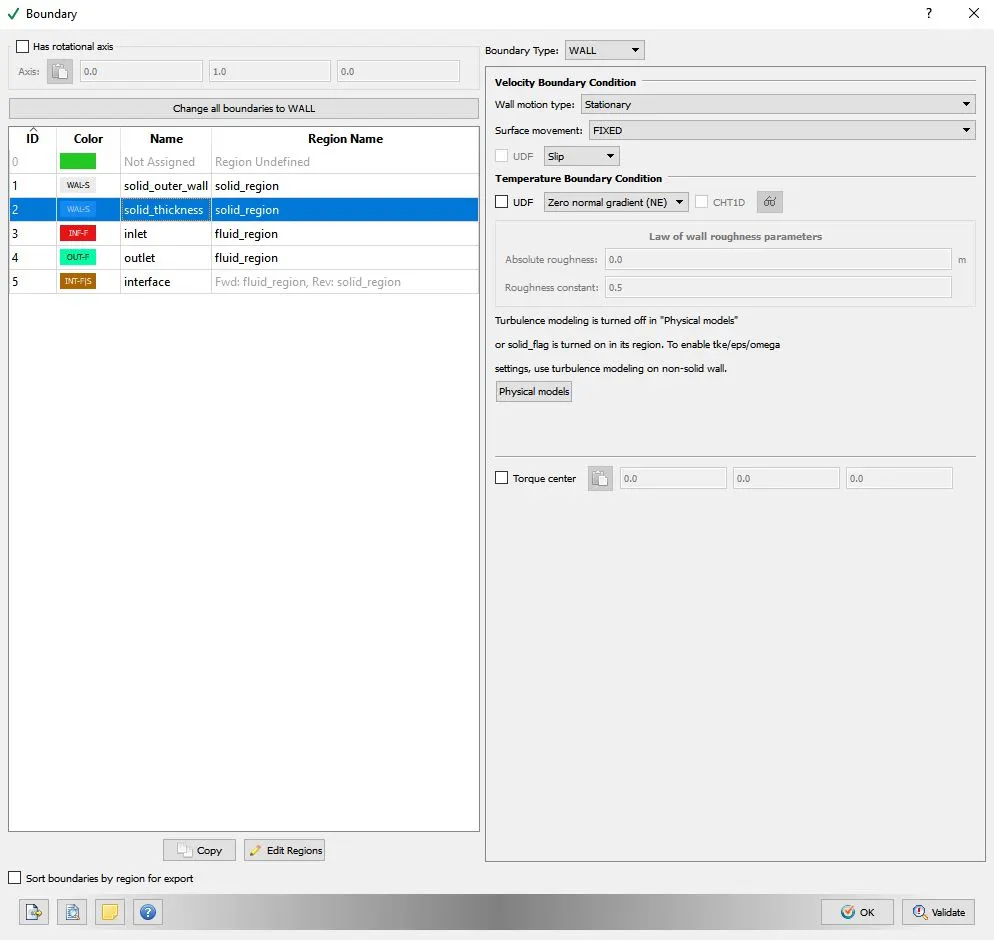
calculating velocity:

Re = (rho*V*D)/(Dynamic viscosity)

>> V=3.7m/s

Initial Conditions and Events:-

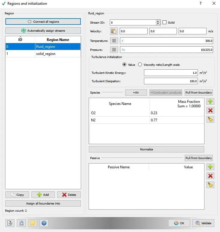
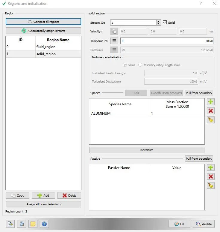
Regions and Initialization:

Physical Models:-

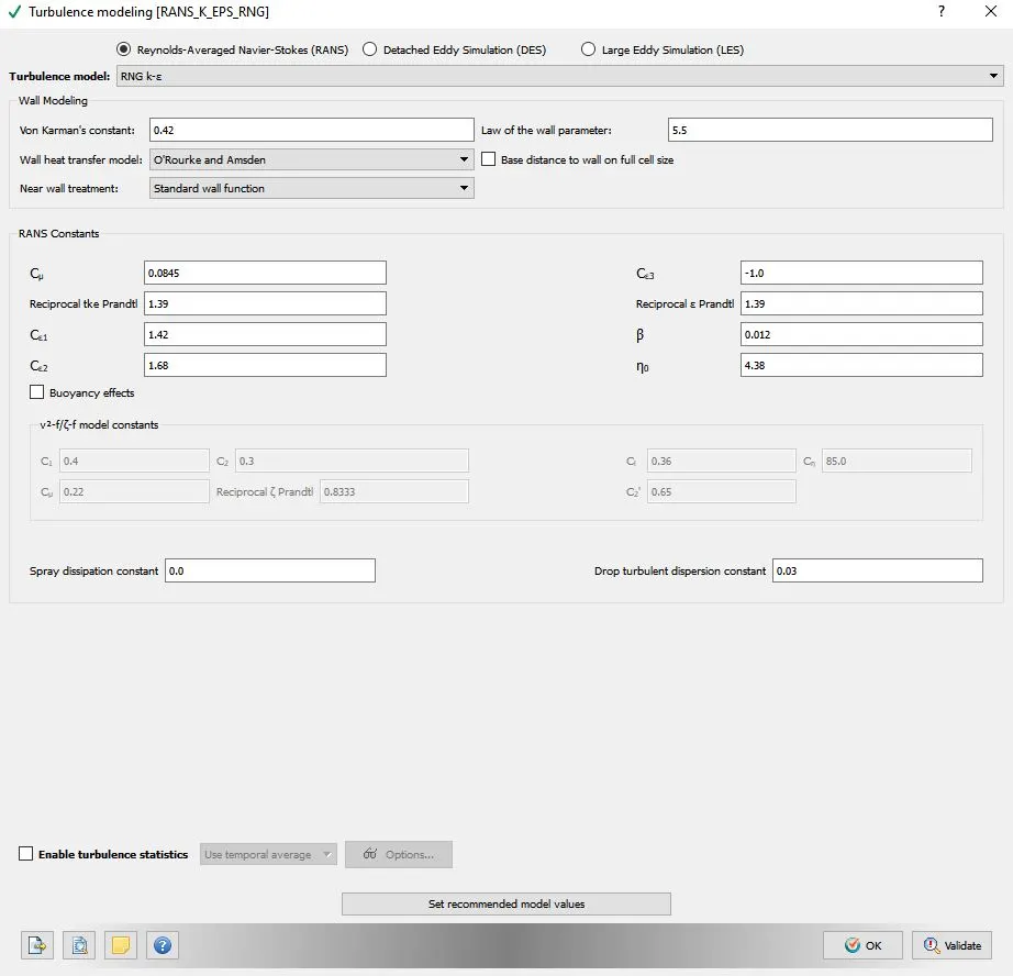
Click on Physical Models > select 'Turbulence Modeling' and 'Super-cycle Modeling' in this case.

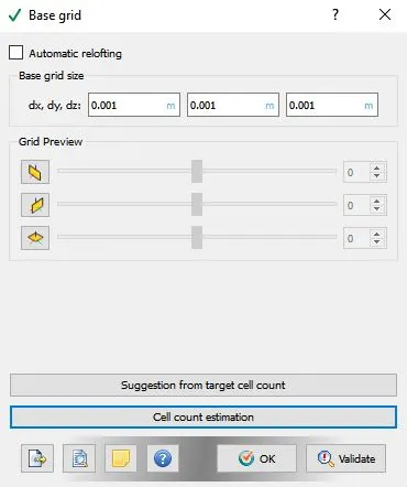
Grid Control: -

Post-Processing: -

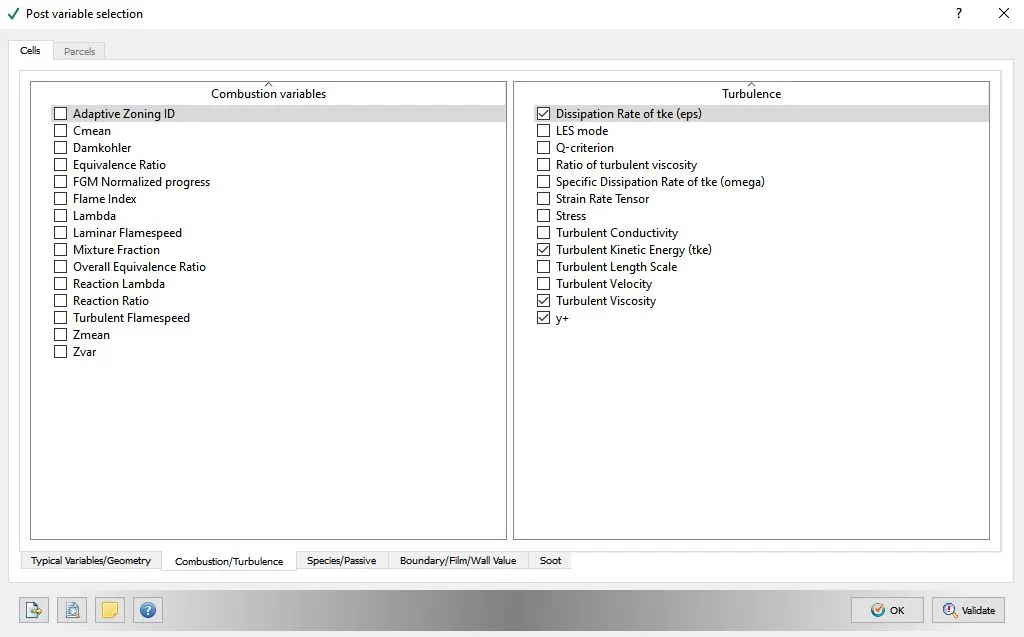
Post Variable Selection:

Click on Typical Variables/Geometry > Select required variables.

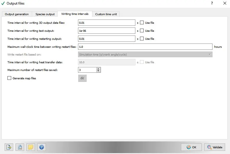
Output Files:

• With this setting up of the case is completed.
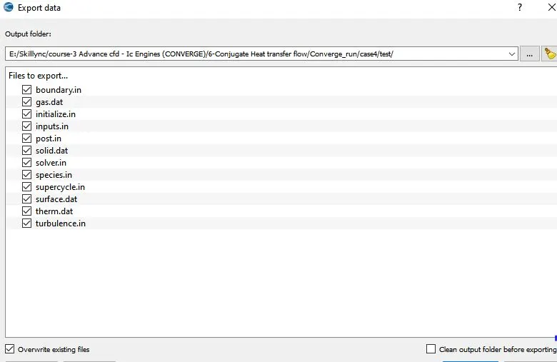
• Now go to File > Export > click on Export Input Files. select the destination folder(test) to save the data.

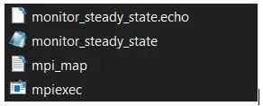
• After importing the input files, paste the "mpiexec.exe file".

• Now open Cygwin and navigate to the location where the setup files are imported.

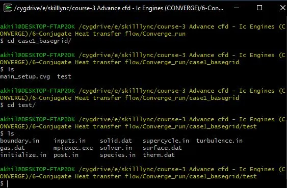
• Once we navigate to the respective folder, we need to run the simulation. To run the simulation, use the following command in Cygwin;

>> Here path is copied from " C:ProgramFilesConvergent_ScienceCONVERGE3.0.15binconverge-intelmpi.exe ".

• Now the simulation starts running, and it displays the steps in cygwin. As the simulation begins it creates multiple folders (i.e. '.scratch' & output) in the path where we saved the input files.

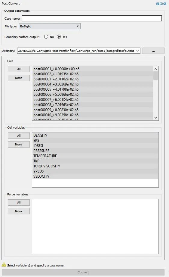
• Once the simulation is complete, to perform post processing we need to convert the obtained result data into format where we can access in Paraview. These converted files are directed to the Output folder.

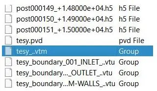
• Open PARAVIEW > direct to folder where the output is saved > select '.vtm(group file)' > data imported to paraview.

• Necessary contours, profiles and animations are generated using paraview. To generate plots we can use ConvergeStudio (line plotting option).
• Hence required plots, contours, animations are obtained in order to study the results.

Geometry:

Case Setup:

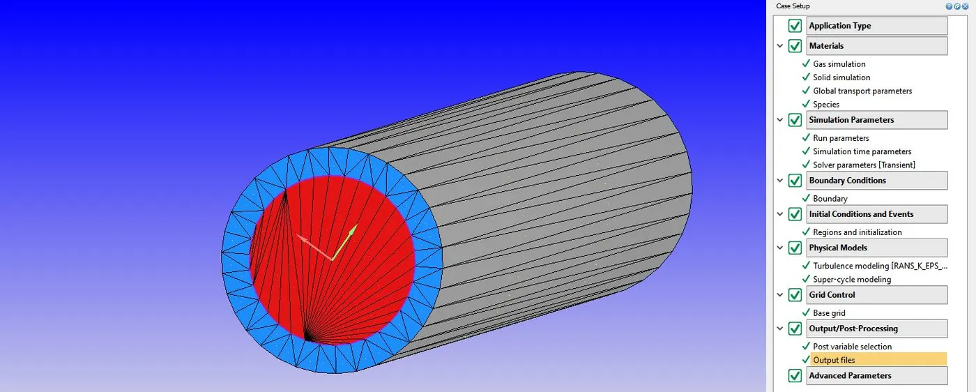
Observations:

To perform Grid Dependency Test (Mesh size-0.004m,0.003m,0.002m)

Case1- Gride size-0.004 and supercyle stage interval-0.05 (Base Mesh)

Mesh:

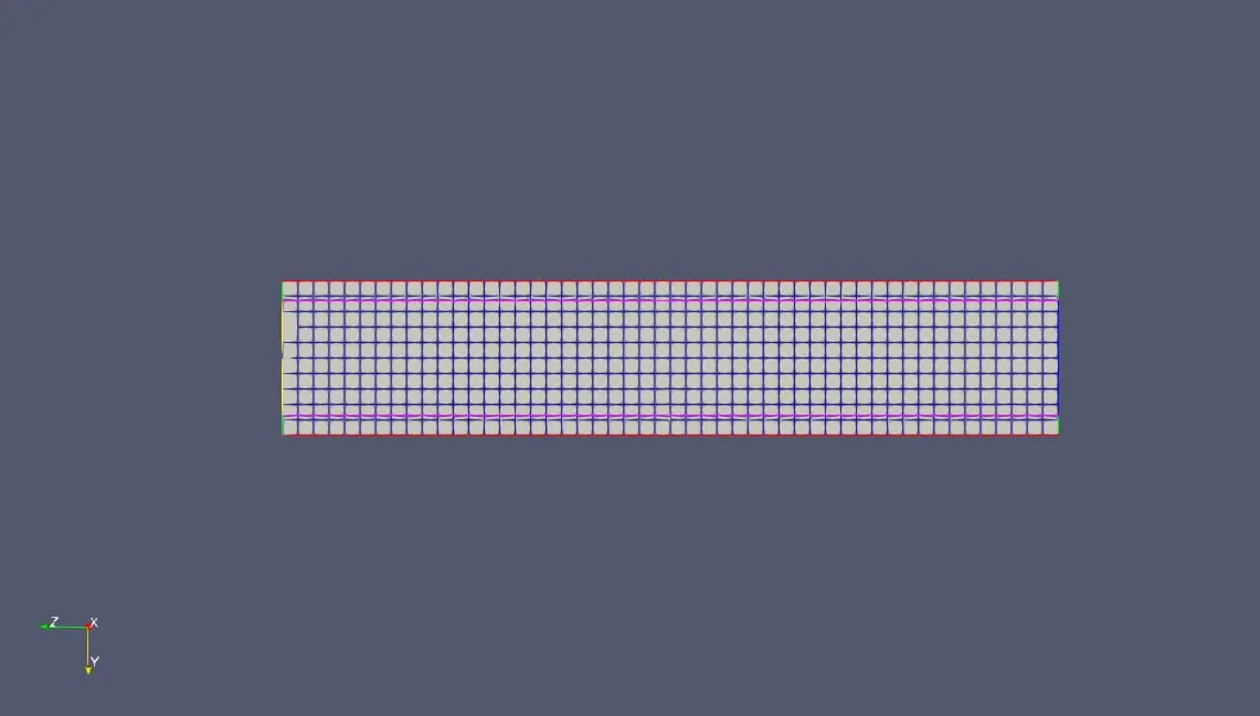
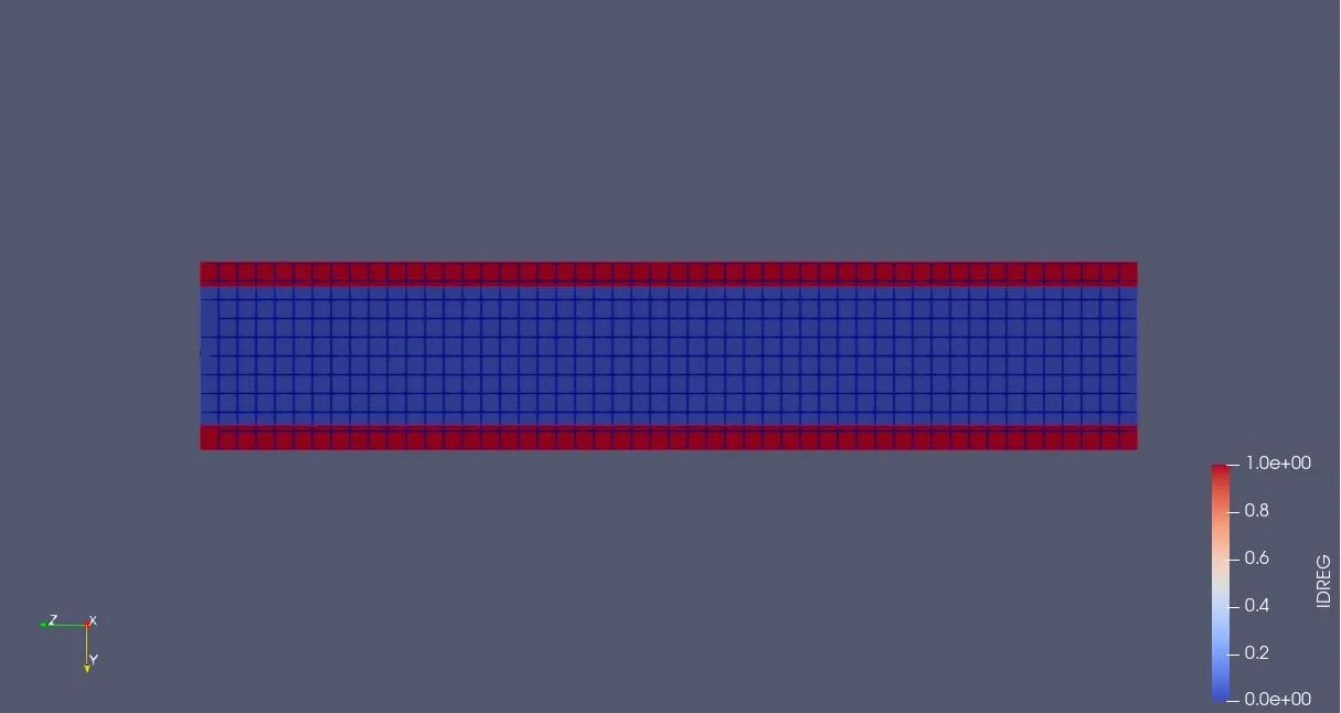
IDREG Contour-

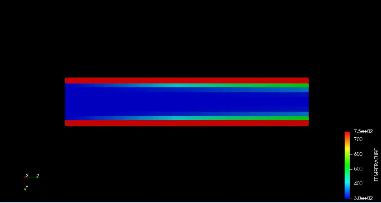
Temperature Contour-

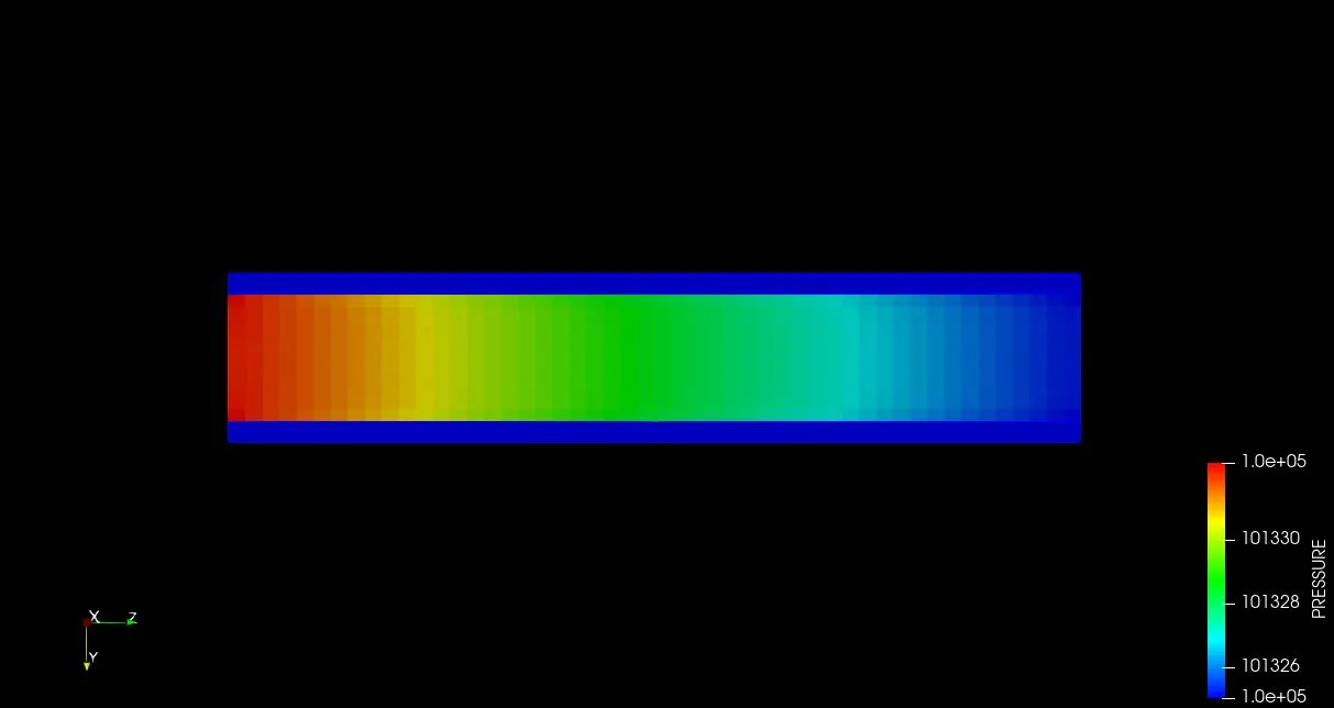
Pressure Contor-

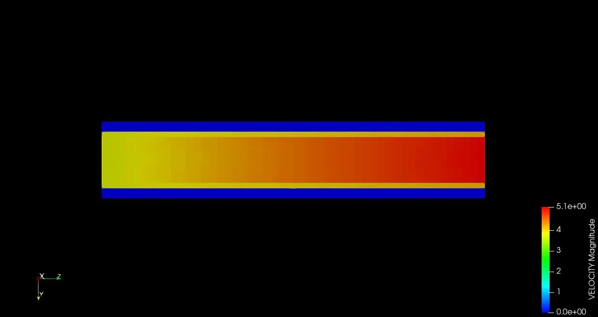
Velocity Magnitude-

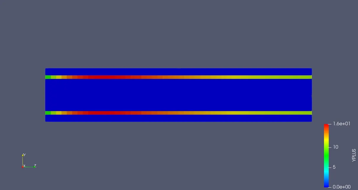
Y+ Contour-

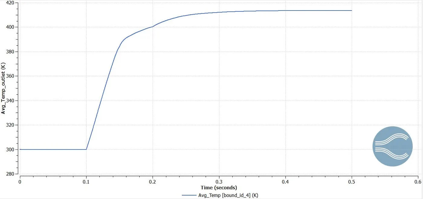
Average Temperature at Outlet plot-

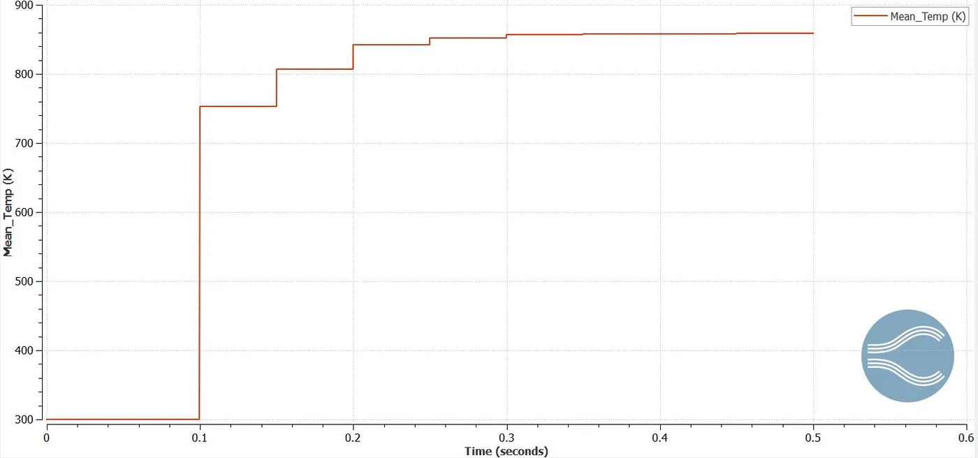
Mean Temperature plot-

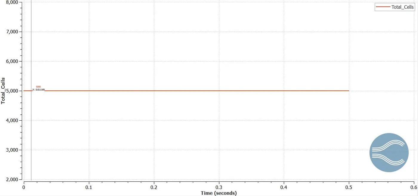
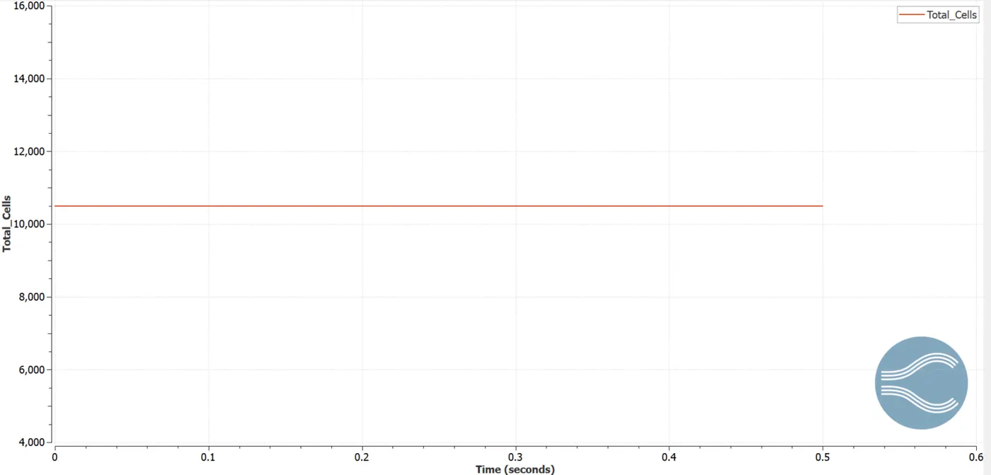
Cell Count-

Animation-

Case-2 Gride size-0.003 and supercyle stage interval-0.05

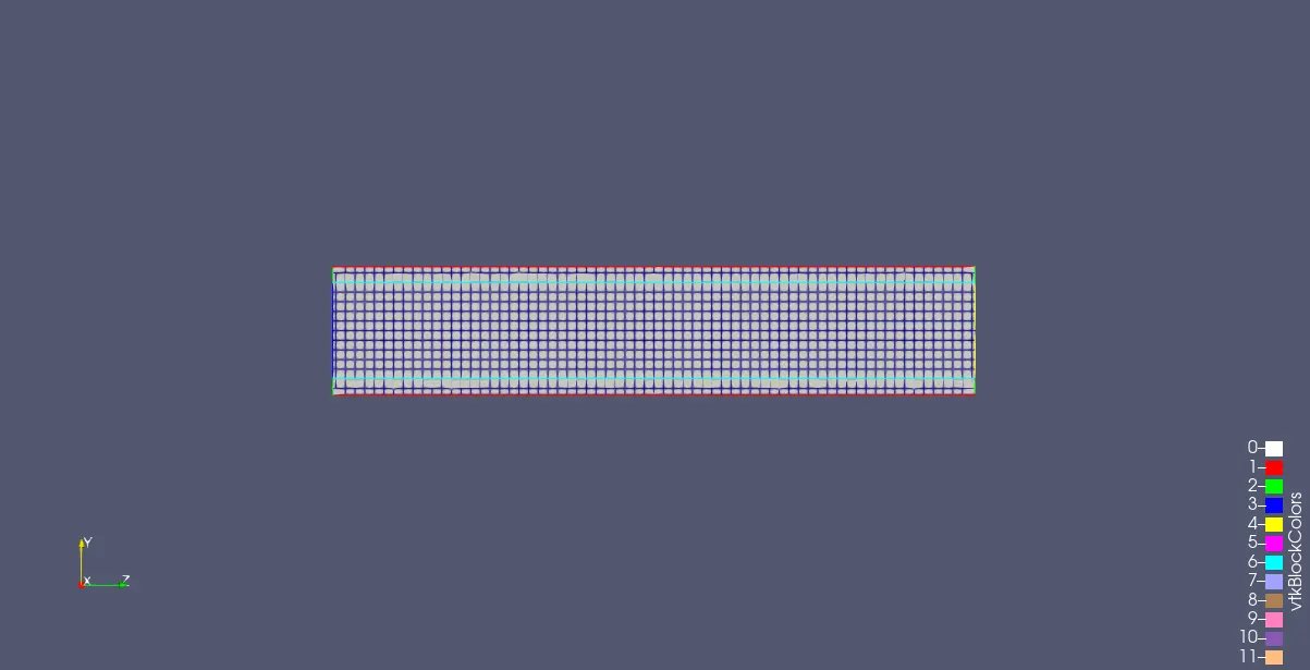
Mesh:

IDREG Contour-

Temperature Contour-

Pressure Contor-

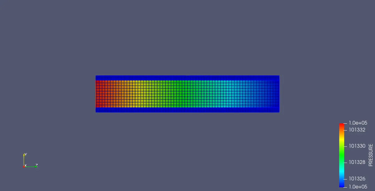
Velocity Magnitude-

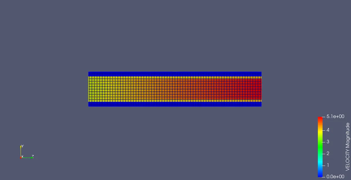
Y+ Contour-

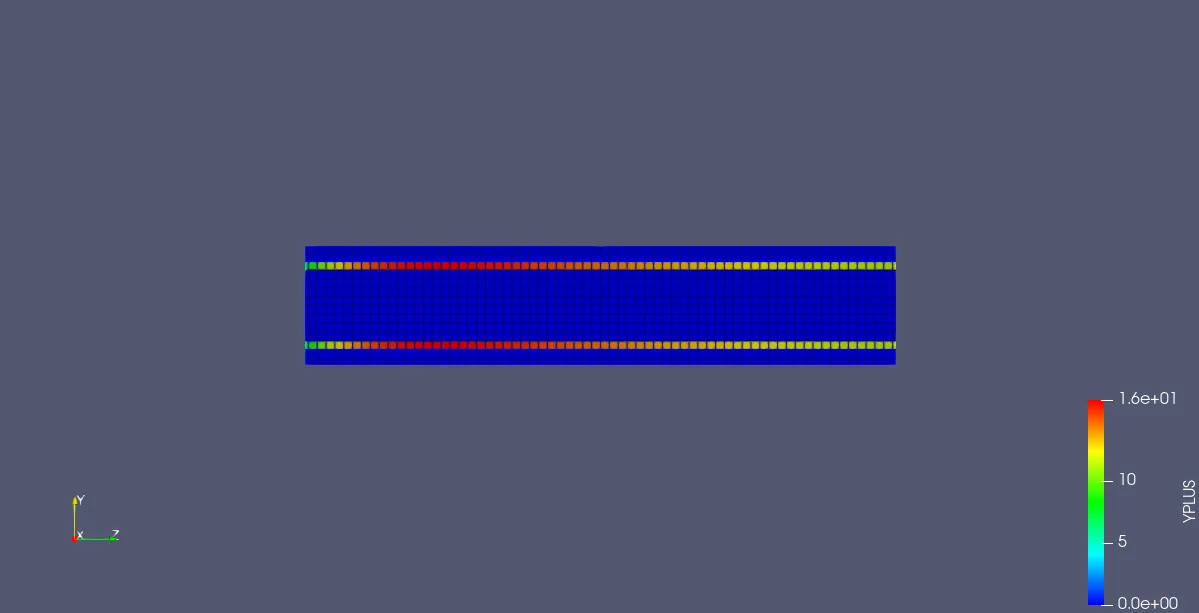
Average Temperature at Outlet plot-

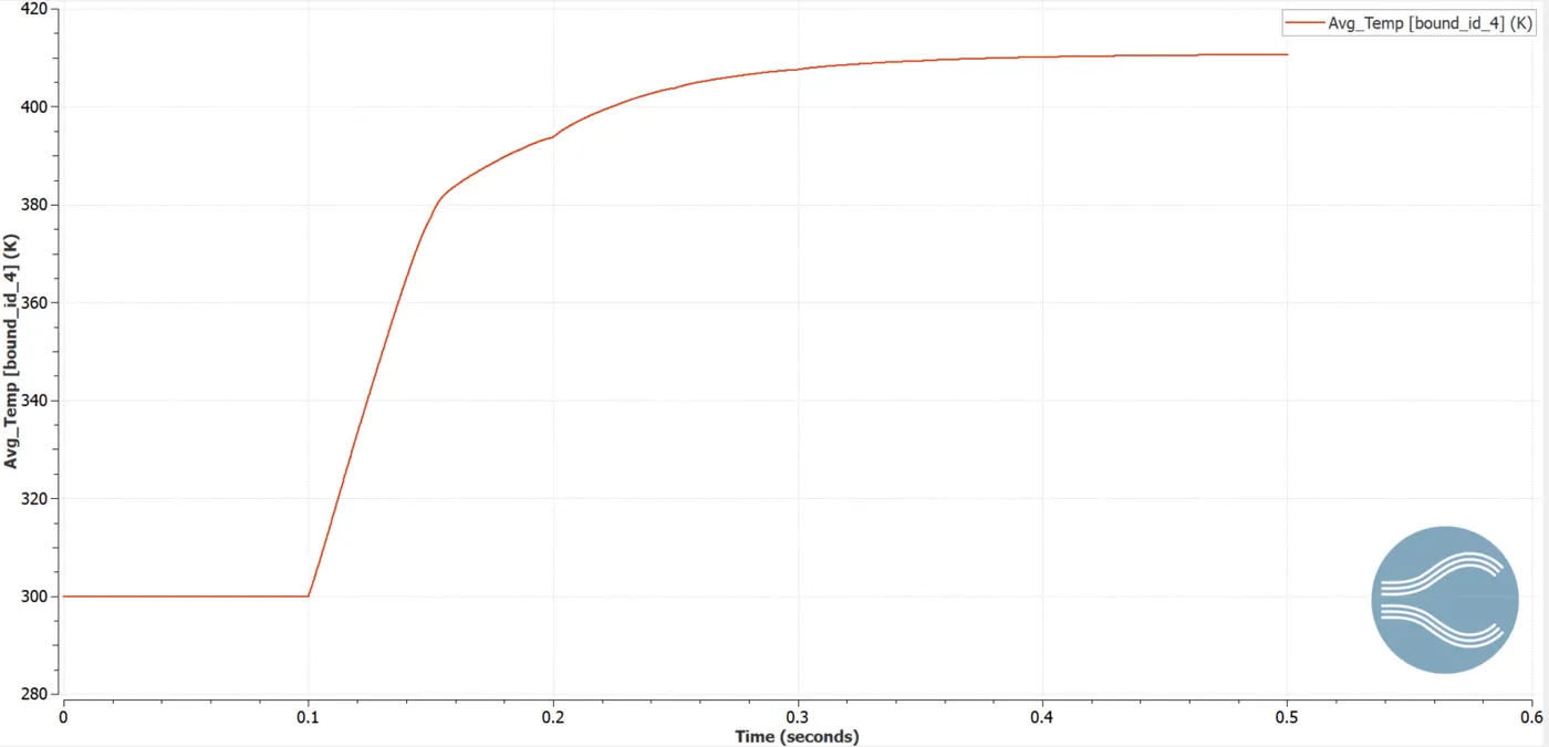
Mean Temperature plot-

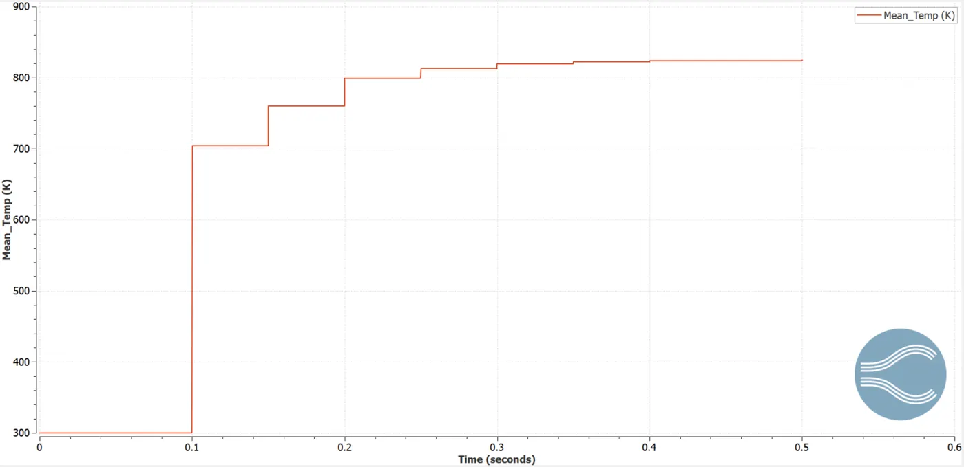
Cell Count-

Animation-

Case-3 Gride size-0.002 and supercyle stage interval-0.05

Mesh:

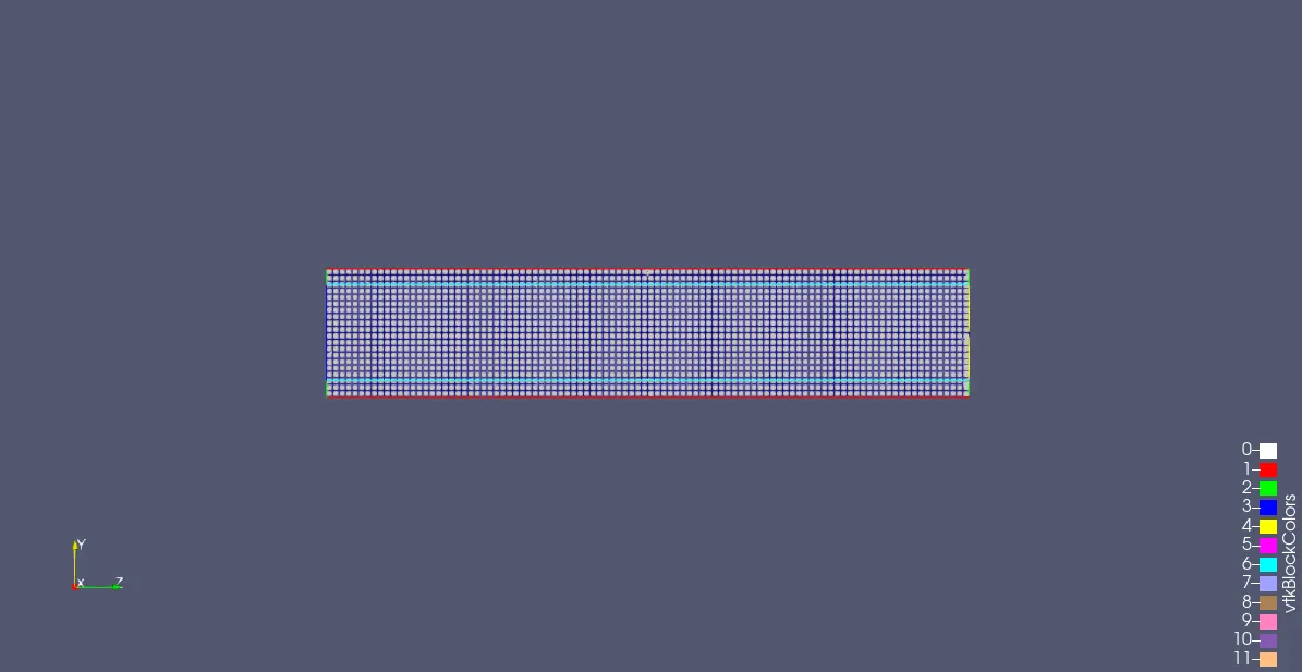
IDREG Contour-

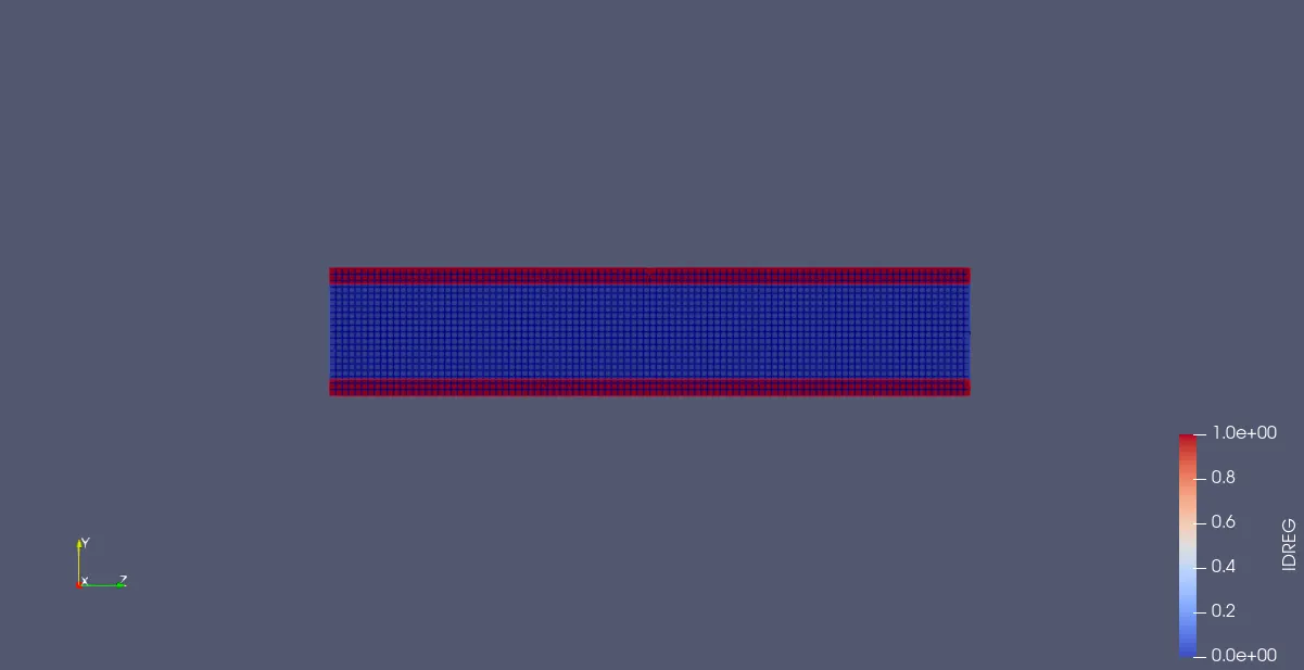
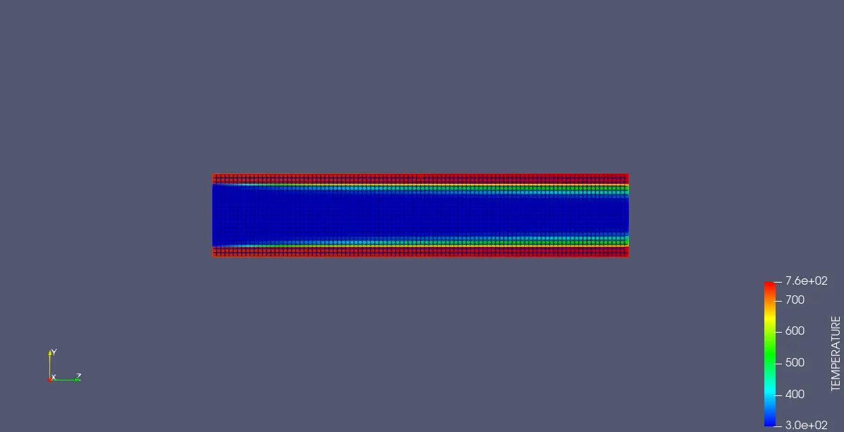
Temperature Contour-

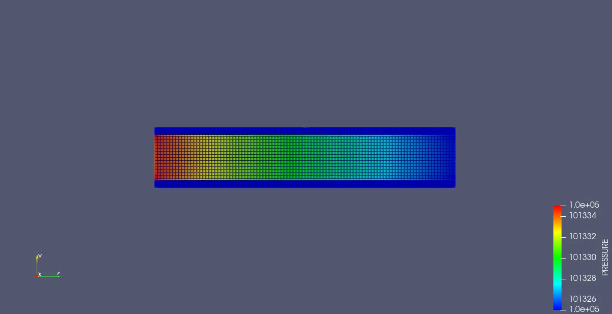
Pressure Contor-

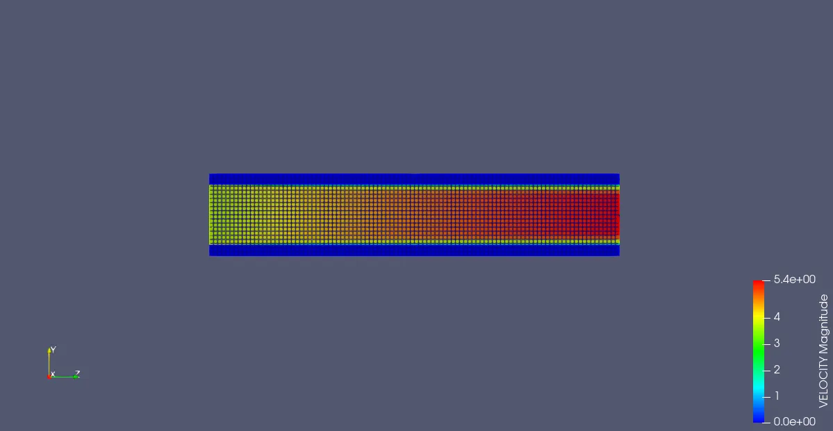
Velocity Magnitude-

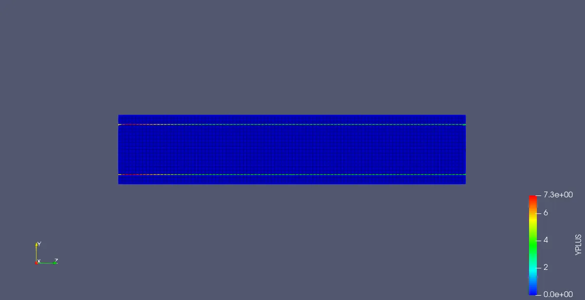
Y+ Contour-

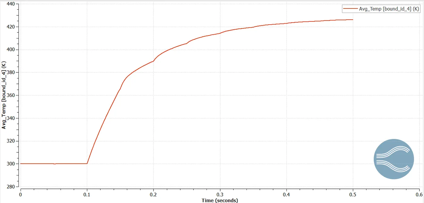
Average Temperature at Outlet plot-

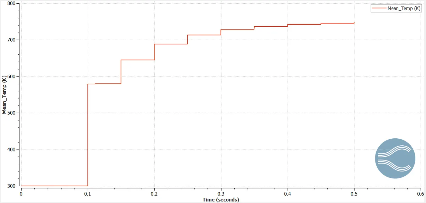
Mean Temperature plot-

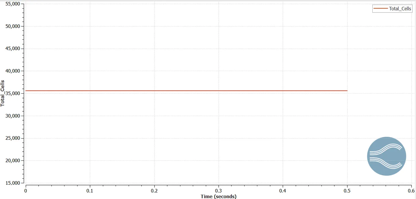
Cell Count-

Animation-

To study the effect of supercycle stage interval.

Case- Gride size-0.003 and supercyle stage interval-0.01

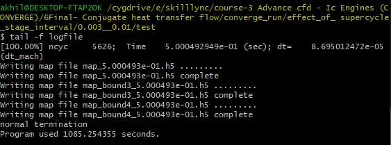
Case- Gride size-0.003 and supercyle stage interval-0.02

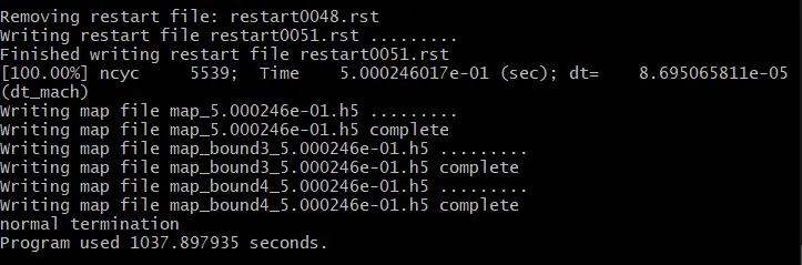
Case- Gride size-0.003 and supercyle stage interval-0.03

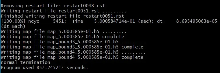
Fluid Region:

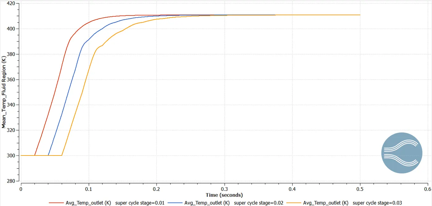
Solid region:

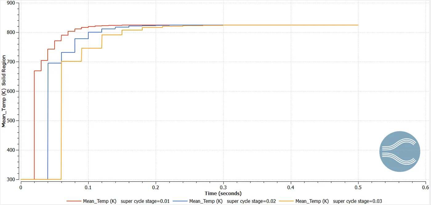
Results:

• Initially for grid size=0.004, it is observed that the mesh is too course.But on performing grid dependency test for various mesh sizes it is clear that for grid size=0.001 the mesh is finel refined. As the cell count is increased for the finer mesh, it takes longer time to run the simulation. Finer mesh gives accurate results.
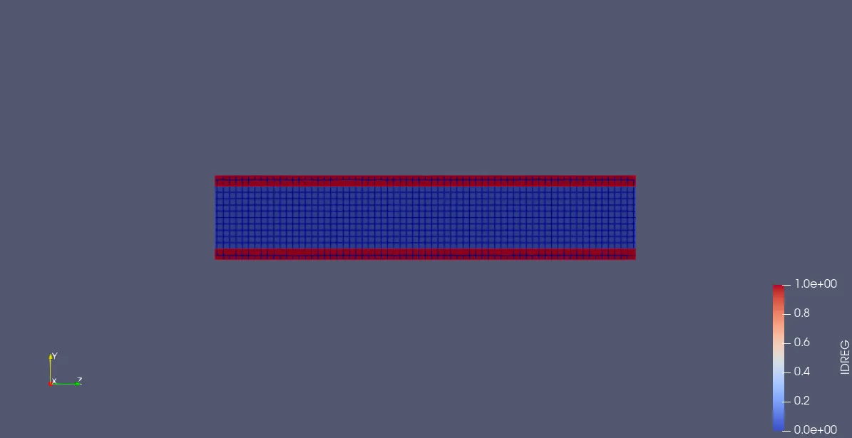
• The IDREG Contour represents the regions of the geometry i.e. from the contour "1"- indicates the solid region and "0"- indicates the fluid region.
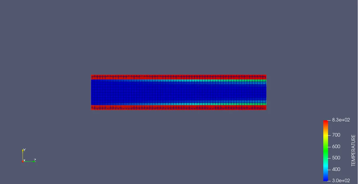
• The study says that the heat transfer starts from the outer side by external heat flux and transfer through the solid region through conduction and for the inner fluid heat is passed by convection.
• From temperature contours, we can notice that the outlet temperature converges to a different values for different grid sizes.
• The Y+ contour clearly shows the changes as the grid size is refining. i.e. as the mesh changes the Y+ value changes.
• As the grid size is decreases the mesh size gets finer and the Y+ alue for the refined mesh also decreases.This can be observed in the y+ contours.
• If the mesh size is decreased, we can observe a small drop in solid region temperature.
• From the second part, it is observed that as the supercycling interval decreases, the simulation time decreases.

Case	Grid Size	Supercyclinng Interval	Run Time (seconds)
1	0.003	0.01	1085.254
2	0.003	0.02	1037.897
3	0.003	0.03	857.245

Conclusion:

• Simulation is setup to study the flow through a pipe. To run the cases velocity is calculated from the given Reynolds number.
• Grid dependency test is performed by maintaining the supercycle stage interval as constat for all the cases. Various contours are generated to show how the temperature is converged for different mesh sizes.
• The Y+ contours are also generated in order to check the changes in values when the grid size is changing or refining.
• The effect of supercycle stage interval is also studied by inspecting the simulation time and the stage interval value.