Week 6: Conjugate Heat Transfer Simulation
Conjugate Heat Transfer Simulation of a pipe
Objectives:
- Setup a conjugate heat transfer simulation of a flow-through pipe and perform a grid independence test for the outlet temperature.
- Compare the simulation time against several supercycle stage intervals.
Conjugate heat transfer:
The term Conjugate heat transfer comes into the picture when heat transfer modes occur simultaneously within and between fluid and solid regions.
In solid region, the following energy equation is solved
`ρ C p ( (∂ T)/ (∂ t) ) = ∇ . ( k ∇ T ) + S h`
and in the fluid region, entire set of Navier Stokes equations are solved
Geometry:
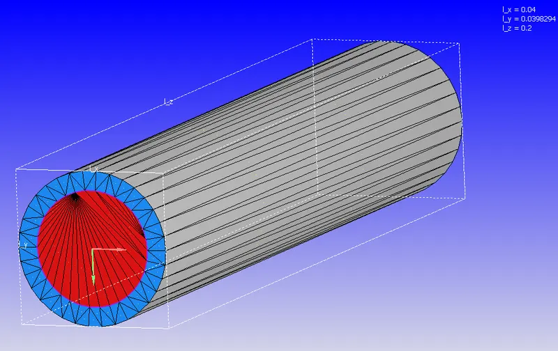
The geometry is a 0.2m long tube with an outer diameter of 0.04m and an inner diameter of 0.03m.
Materials:
Fluid - Air
Solid - Aluminium
Simulation setup:
Simulation Type: Transient
Solver: PISO-Density based
Turbulence Model - ON, K-epsilon
Run parameters:
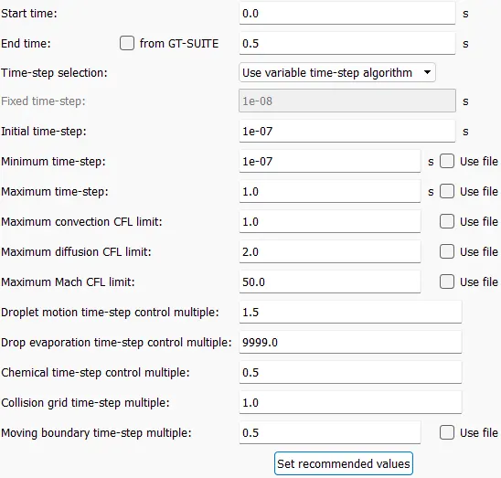
The simulation is set to capture the phenomenon for 0.5s with an initial and minimum time step of 1e-07s and a maximum time step of 1.0s. Maximum convection and diffusion CFL limits are set to 1 and 2 respectively.
Boundary Conditions:
| Boundary | Conditions |
| Solid Outer Wall | Fixed wall, Heat flux 10000 W/m2 |
| Solid Side (Thickness Zone) | Wall |
| Inlet | Inflow, Velocity - 0.3516 m/s (Re=7000) |
| Outlet | Outflow, Ambient Pressure-101325.0 Pa |
| Fluid and Solid Interface |
Interface, Fluid region - Law of Wall applied to both velocity and temperature. Solid region - Slip |
Initial Conditions:
Region 0 - Fluid (Air at T=300K, P = 101325 Pa)
Region 1 - Solid (Aluminium at T=300K)
Super cycling:
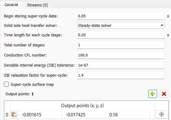
In super-cycling, the fluid solver is frozen periodically while the heat transfer in the solid is allowed to progress to steady state.
Grid Generation:
In this study, the Grid Independence test is performed in order to obtain the suitable grid size which yields the correct result at a reasonable computation time.
A uniform grid size of 0.002m to 0.0015m is iterated to achieve a suitable result.
Results:
Grid Independence Test:
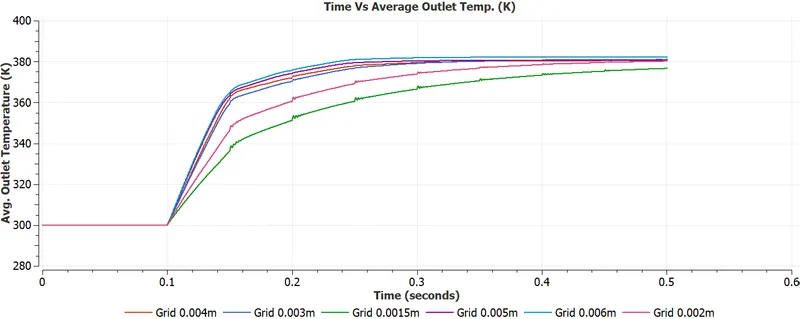
In the above plot, variations of average outlet temperature with respect to several grid sizes are shown. It is clear from the plot that the grid size of 0.0015m and 0.006m diverges from the accurate value. Other grid sizes from 0.002m to 0.005m converge almost to a similar value. Hence it is ideal to consider the grid which gives a suitably accurate value at the expense of least computation time. In this context, a grid size of 0.005m fulfills the necessity.
Baseline Configuration (0.005m):
Grid:
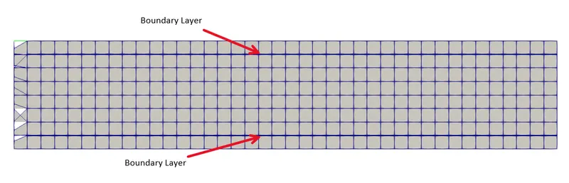
The above grid is formed with a size of 0.005m. The boundary layer is the fluid region that is formed next to the wall which has zero velocity. In order to visualize the boundary layer effectively, much finer cells have to be accommodated. The marked regions on the above figure are the regions where boundary layers are formed and hence there is a fine layer of mesh across it.
Velocity: (Click here)
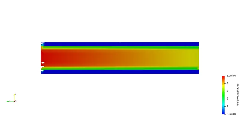
The velocity contour shows the flow through the pipe. At the inlet, the velocity is high and then it reduces as it progresses.
Pressure: (Click here)
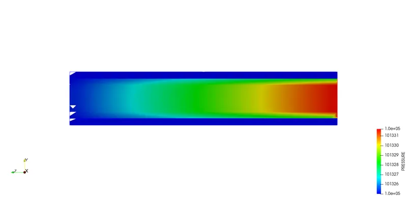
Pressure contour is in accordance with the velocity plot in an inverse relation.
Temperature: (Click here)
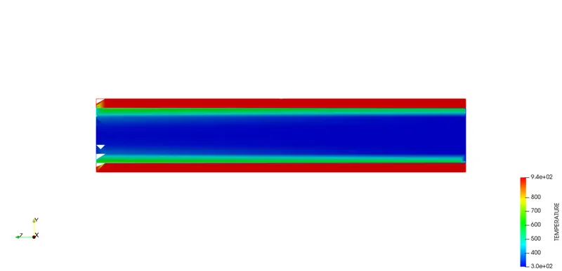
Above temperature, contour shows the heat transfer from the solid wall into the fluid domain. The heat flux transfers through the wall and then the molecules of the fluid region near the wall reach a higher temperature.
Y+ : (Click here)
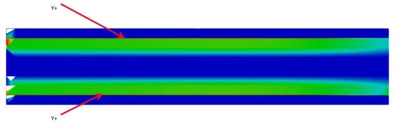
The behavior of the flow near the wall is a complicated phenomenon and to distinguish the different regions near the wall the concept of wall  has been formulated. Thus is a dimensionless quantity, and the distance from the wall is measured in terms of viscous lengths. In the above figure, Y+ near the wall is higher and it decreases radially as velocity increases into the mainstream flow.
Effect of Supercyling:
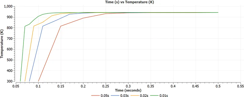
In the above plot, the variation between Supercycling interval and Temperature is shown. The temperature reaches a steady-state in the case of a higher supercyling interval. This is because the solver which handles heat transfer across solid regions does not reach the steady-state within the provided short interval. The time taken to compute each intervals are shown below;
| Case | Supercycle interval (s) | Time (s) |
|
Baseline Grid 0.005m |
0.05 (baseline) | 127.195249 s |
| 0.03 | 130.988147 s | |
| 0.02 | 132.652247 s | |
| 0.01 | 137.464650 s |
Inferences:
- The most efficient grid size is 0.005m in terms of both computational effort and accuracy.
- Supercycling overcomes the time-scale disparity between fluid and solid regions. The lower the super cycling interval, the higher the computation time. Hence an optimum level of the time interval has to be chosen such that the solver which solves the solid heat transfer becomes steady.
References:
[1] https://www.engineeringtoolbox.com/reynolds-number-d_237.html