Week 6 - CHT Analysis on a Graphics card

Aim: Analysis of steady-state conjugate heat transfer using a graphics card model

Objectives :

1. Run the simulation by varying the velocity from 1m/sec to 5m/sec for at least 3 velocities and discuss the results.
2. Find out the maximum temperature and heat transfer coefficient attained by the processor.
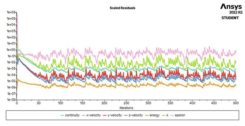
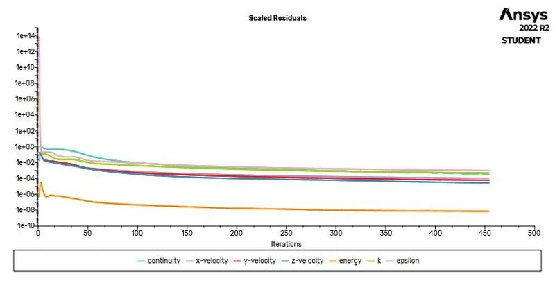
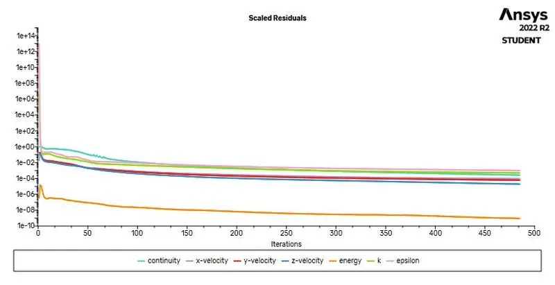
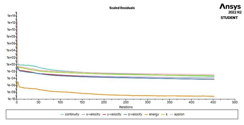
3. Prove that the simulation has achieved convergence with appropriate images and plots.
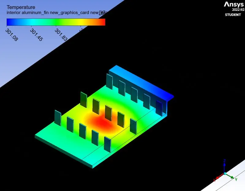
4. Identify potential hotspots on the model.

Introduction:

Conjugate heat transfer analysis addresses the heat transfer between a body and a fluid running over or inside it as a result of interaction between two objects. It is based on a mathematically structured problem. The details of the temperature distribution and heat flux along the interface at the matching interface eliminate the need to calculate the heat transfer coefficient. Additionally, it is possible to determine the heat transfer coefficient later.

Numerical approaches are one of the simplest ways to realise conjugation. Iterative methods are used to set and solve the boundary conditions for the interface between a fluid and a solid. Other than by using the hit-and-miss approach, there is no way to make accurate assumptions about the values of the initial boundary condition for convergence.

Application:

The conjugate heat transfer methods have improved as a modelling and research tool for engineering systems and natural phenomena in a variety of fields, such as aerospace and nuclear reactors, thermal goods processing, food processing, complex medical procedures, ocean thermal interaction, and metrology.

Through the design of heat sinks and heat exchangers for the waste treatment plant, CHT has greatly improved the cooling performance of electronic equipment in recent years. The exhaust port system is one such CHT use.

Solving & Modelling approach

• Graphic card file is loaded into the spaceclaim
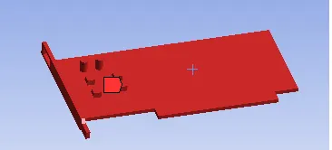
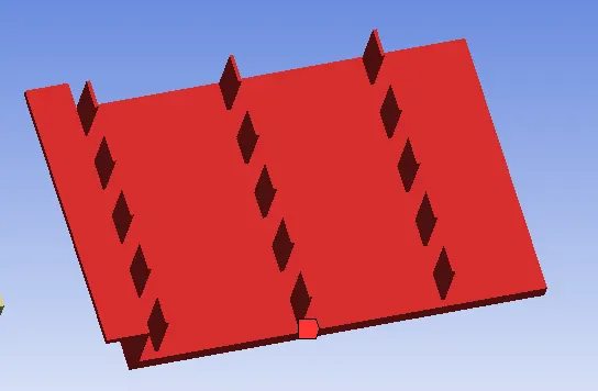
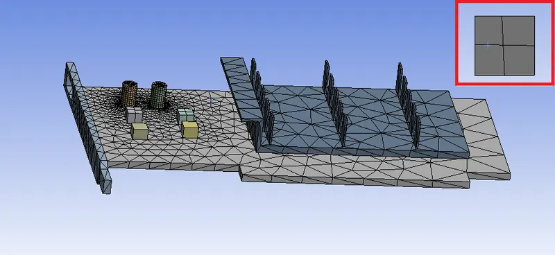
• The graphics card consists of a processor, PCB base, aluminum fin base, memory cards, and capacitors.
• The solid and liquid volume under consideration are both necessary for CHT analysis, and Spaceclaim offers a volume extract option for choosing edges for fluid volume. In this case, the solid and liquid volume under consideration are air and the components of the graphics card.
• the underlying theory of how air carries away the heat produced by the CPU. The aluminium fin is utilised to increase the heat transfer surface area.
• The share topology is configured to make the mesh conformal and to lower interpolation error.
• The meshing window is then loaded, where the named selection is made and the baseline mesh and refined mesh are set.
• The construction of the material is chosen with the fluid material and the solid material separated.
• To comprehend the behaviour of temperature, velocity, and surface heat transfer coefficient at the interface, the relevant contour images and graphs are reviewed.

Preprocessing and solver setting

Baseline Mesh

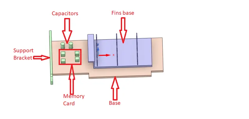
To make the mesh conformal and to lower interpolation error, the share topology is developed.
The baseline mesh of 0.01 mm is generated after the geometry has been imported into the meshing interface.
For the graphics card interface, the named decision is made.

Inlet velocity (1 , 2.5 , 5 ) m/sec

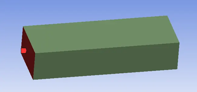
Outlet

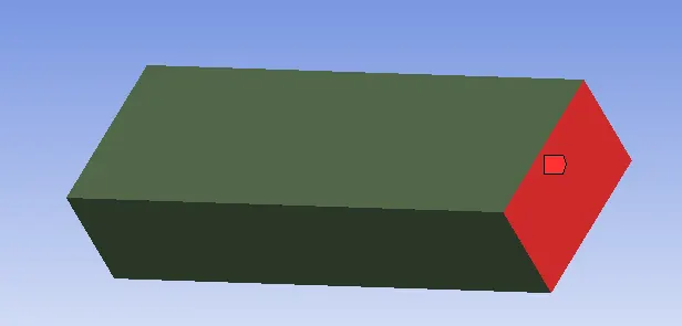
Symmetry Wall

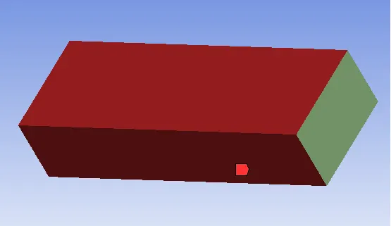
Graphics card base (Wall)

Aluminum fin base (Wall)

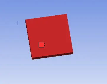
Processor (Wall)

Physics setting

Reference data

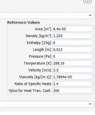
Turn on the energy Equation as temperature is involved in the problem

Viscocity

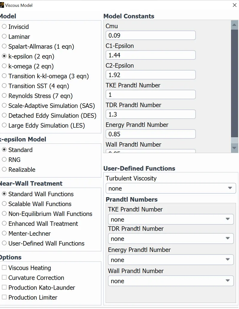
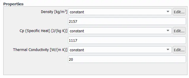
Material Properties

Fluid

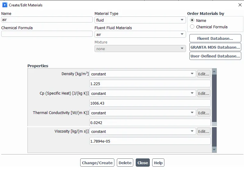
Solid

Processor

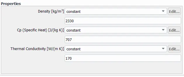
Aluminum Fin Base

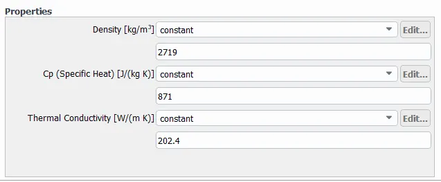
Graphic card Base

Cell Zone

The processor wall is selected in the zone tab's edit option, the source term is enabled by choosing one source, and the volumetric heat source value of 5e7 w/m3 is entered as a constant. This equates to 150 W, which is sufficient for the majority of graphics cards but necessitates more for cards like the Nvidia RTX, which needs more than 320 W and a system power of 750 W. Since most mid-range cards only require 150 W, these typically have a 6 pin power connector. GPU power connectors are discussed in https://www.gpumag.com/.

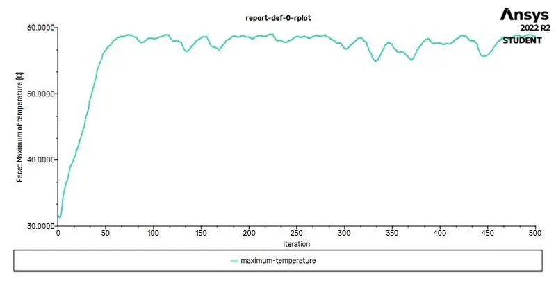
Selecting the processor wall results in the creation of the maximum temperature plot.

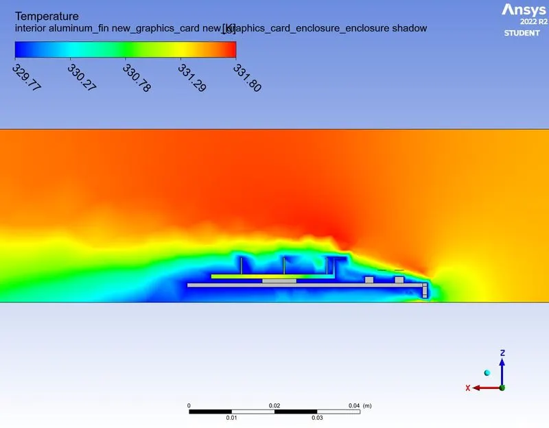
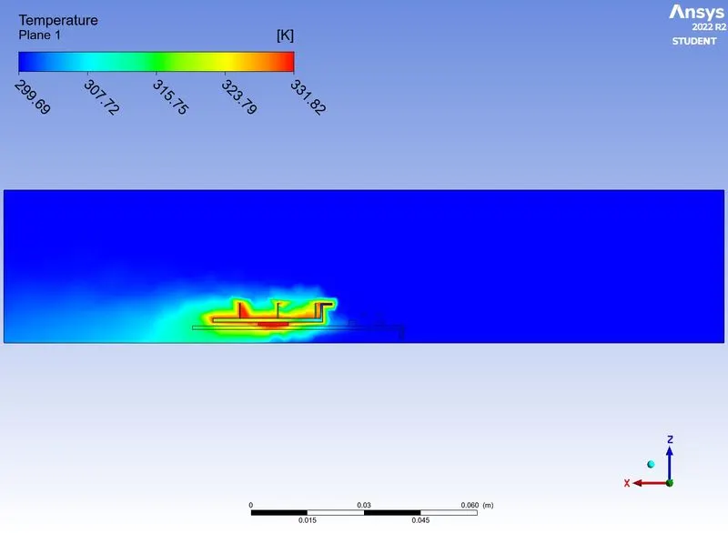
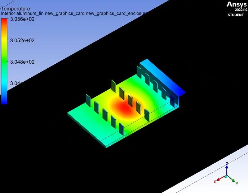
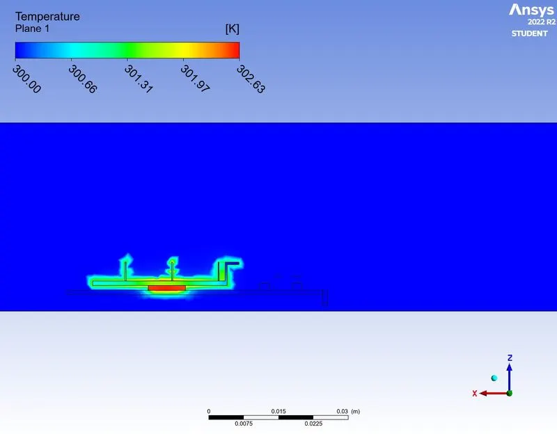
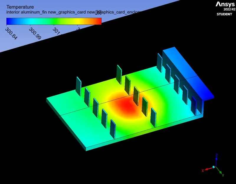
The complete graphics card zones are chosen to generate the temperature contour.

Meshing:

It involves employing the finite volume approach to discretize the entire volume. You can carry out the steady-state solution by choosing "SIMPLE", "SIMPLEC", or "COUPLED". Since the baseline mesh is coarse, the momentum for the connected scheme is first order upwind; however, for the refined mesh, the pressure, momentum, and energy are all of second order. The "Least Square Cell-Based Scheme" is chosen to use the gradient. In order to increase numerical accuracy and bring the solution closer to convergence, body sizing and edge sizing methods are used for the refined mesh.

Case-1

Element size: 0.01m">0.01m

Inlet velocity: 1msec">1 m/s

Number of element: 83919

Number of nodes: 15734

Pressure-velocity coupling scheme: Coupled

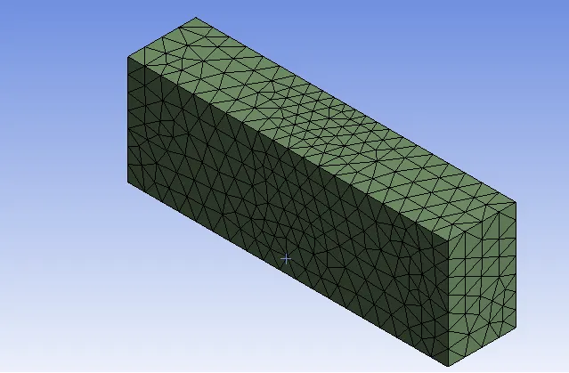
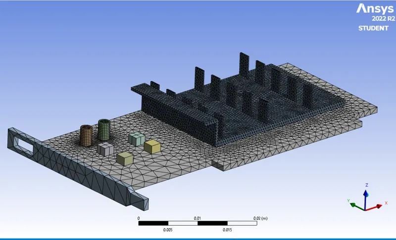
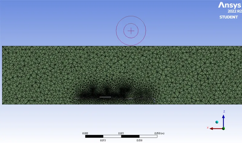
Enclosure mesh

Graphic card mesh

Plot Results

Residual Plot

Maximum of temperature plot

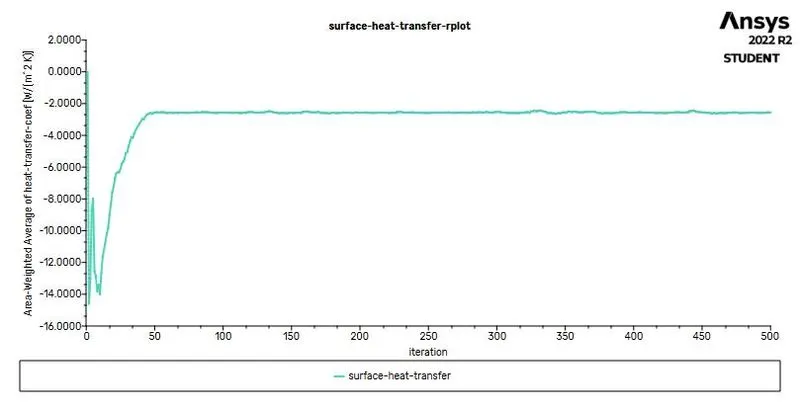
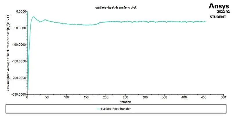
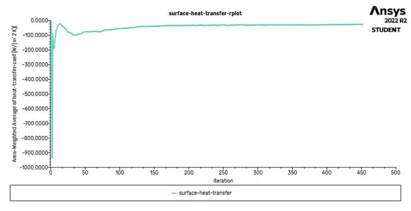
Heat Transfer co-efficient

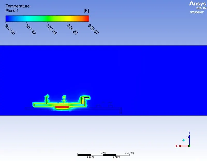
Temperature contour

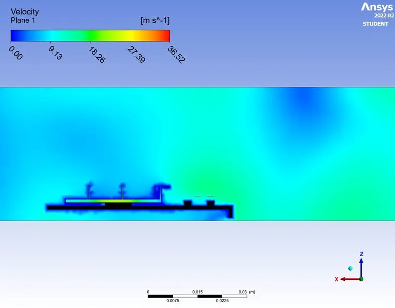
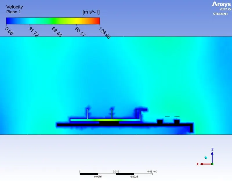
Velocity contour

Refined Mesh:

A. MESH

1.Element Order: Linear

2.Element size: 0.003 m

3. Body Sizing (Fin)

• Element Size: 0.0005 m
• Curvature Capture: Yes

4. Body Sizing (Processor)

• Element Size: 0.0005 m
• Curvature Capture: Yes

5. Body Sizing (Base)

• Element Size: 0.003 m
• Curvature Capture: Yes

6.Number of Nodes: 87866

7.Number of Elements: 497438

B.Simulation setting

The simulation configuration was chosen using the same criteria as the initial mesh. The change in the inlet velocities will only affect the simulation's output.

Results at 1m/s velocity

C. Residual output

D. Heat transfer co-eff

E. Max temperature

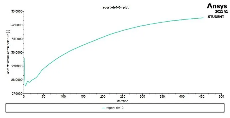
max temperature for 1 m/s

Facet Maximum [C]

-------------------------------- -------------------

interior-processor 32.531915

Temperature Contour

Velocity contour

Results at 3 m/s velocity

A. Residual plot

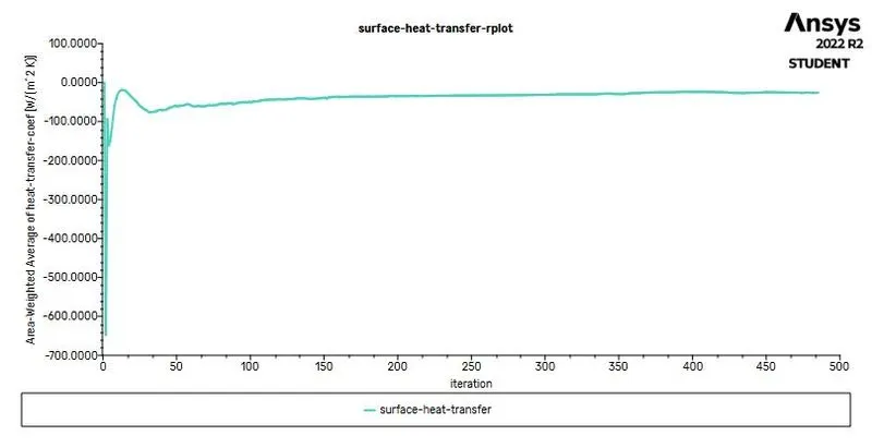
B. heat transfer co-eff

C. max temperature

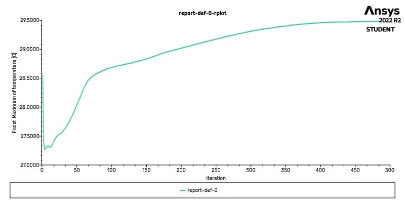
Facet Maximum [C]

-------------------------------- -------------------

interior-processor 29.482111

Temperature Contour

Velocity contour

Results at 5 m/s

Residual plot

heat transfer co-eff

Max temperature

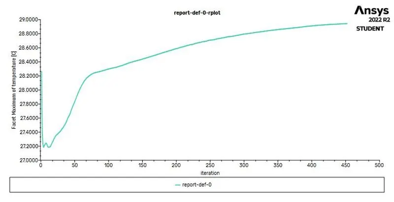
Facet Maximum [C]
-------------------------------- -------------------
interior-processor 28.944025

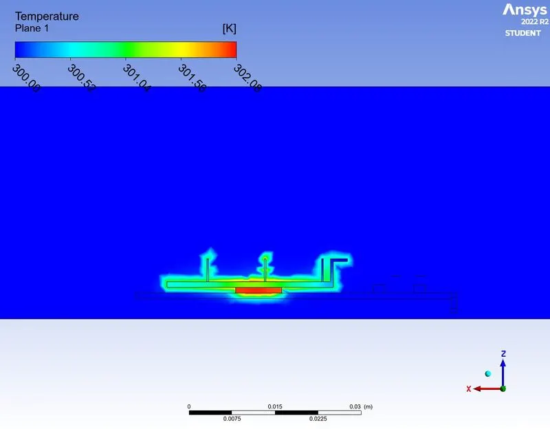
Temperature contour

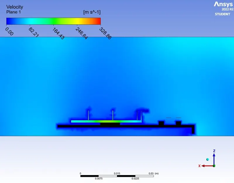
Velocity Contour

Results at glance

Velocity (m/s)	1	3	5
Temperature at proccesor (C)	-1.8348441	-9.7114714	-8.8510126

Conclusion

• As the number of elements rises, precise temperature distribution data are achieved.
• It is apparent from the preceding data that as inlet velocity increases, the net temperature of graphics card components falls.
• As a result, it can be concluded that a higher inlet velocity leads to better cooling and a lower average temperature, protecting the components from harm.
• Thus, it can be concluded that better cooling and lower throttling are caused by a higher inlet velocity. Furthermore, it is evident that components' temperatures rise as inflow velocity drops from 5 m/s to 1 m/s, further demonstrating that higher velocity improves cooling. e average temperature prevents harm to the components.
• we can see from the heat transfer co-efficient graph there is negative value appears because of the heat flux has a different direction with the defined driving temperature difference.