Conjugate Heat Transfer Analysis on a Graphics card (GPU)
Objective:
Perform a steady-state conjugate heat transfer analysis on a model of a graphics card. You can use appropriate materials of your choice for the simulation. Make sure to properly define the correct solid and fluid zones. Refer to the video for further clarification and the model is provided below the video.
Run the simulation for the best possible mesh with a combination of coarse and refined mesh in different regions. Explain the reason for choosing the particular mesh settings.
Mains:
- Run the simulation by varying the velocity from 1m/sec to 5m/sec for at least 3 velocities and discuss the results.
- Find out the maximum temperature and heat transfer coefficient attained by the processor.
- Prove that the simulation has achieved convergence with appropriate images and plots.
- Identify potential hotspots on the model.
Solution:
What is the conjugate heat transfer analysis in a system?
Conjugate heat transfer is a type of heat transfer analysis between solids and fluid(s). This type of heat transfer includes both convection (between fluids) and conductive (between solids) heat transfer, as well as both forced and natural convection. Common applications and use cases of this thermal simulation type include electronics cooling, heat exchangers, industrial machinery, some AEC cases, and more. In order to demonstrate best practices for this application type, an electronics cooling application will be used as an example.
Our project focuses on electronics cooling performance, as the CHT simulation type is most commonly used for this type of application. We will explain how to set up the analysis on the Ansys-FLUENT platform, what guidelines to follow to guarantee success, how to make sure our results are good, and how to make sure your solution is fully converged.
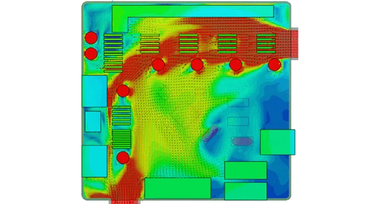
The above picture shows the heat flow over the heat sink in an inlet in an electronics circuit board. Mostly we use electrical appliances or systems.
we are going to set up a simulation where we are going to run it on the graphics processor unit GPU of a computer system. To investigate the conjugate heat transfer analysis for heat sinks that are being used in electronics cooling. This involves the combined fluid flow analysis by
making use of CFD equations and heat transfer analysis, considering separately convection process in fluid flow region and conduction heat transfer in the solid region.
To carry out heat transfer analysis for different fin configurations considering the conduction heat transfer from the base plate to heat fins.
3. To conduct computational fluid flow analysis for different fin configurations, for a fluid part, by solving Navier-Stroke equations to get velocity vectors, pressure contours, and temperature fields for given inlet air velocity. Any Standard RANS model is adopted to account for the turbulence phenomenon. The temperature field is used to get the quantity of heat dissipated or carried away by convection.
4. To determine the heat transfer coefficient, Thermal resistance, and Pressure drop through numerical to predict the thermal performance of a fin for different geometrical configurations.
5. To select the best heat sink with suitable fin geometry for lower thermal resistance, higher heat transfer coefficient, and minimum resistance.
Governing Equations in CFD
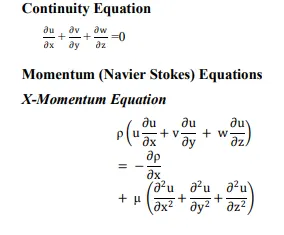
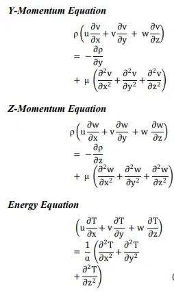
There are mainly three equations that we solve in computational fluid dynamics problems. They are continuity equation, momentum equation, and energy equation. These three equations are collectively called Navier Stokes equations. The flow of most fluids may be analyzed by mathematically solving the last two equations. These three equations represent the conservation of mass, momentum, and energy respectively. These three equations are represented below.
Now we are going to set up the case from space claim and we run for 2 cases where one is base mesh and another one is refined. So we're going to run for base mesh with default element size. In addition to that, we are going to extract the model first.
before we jump into setting up the geometry we need to decide the technical properties of the materials we are going to select. We have ALuminium, Silicon, ABS Thermoplastics.
Silicon Aluminium ABS Thermosplastics
1. Density (Kg/m^3) 2330 2719 1060
2. Specific Heat at Constant pressure(Cp)J/Kg-K 700 871 2001
3. Thermal Conductivity(W/m-K) 130 202.4 0.1
4. Fluid - Air
Density: 1.225(Kg/m^3)
Specific heat Cp J/Kg-K: 1006.43 J/Kg-K
Thermal Conductivity: 0.0242(W/mK)
Viscosity : 1.789e-05 (Kg/ms)
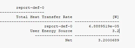
Heat generation takes place at microprocessor at 5e^7 W/m^3
Running the simulation for best possible mesh with combination of coarse and refined mesh in different regions. Explain the reason for choosing the particular mesh settings.
CASE 1: Base Mesh (Coarse)
Now we run space claim and begin setup and while doing so we are going to enable SHARE TOPOLOGY
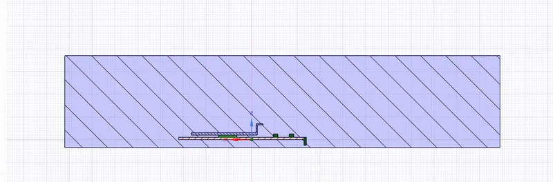
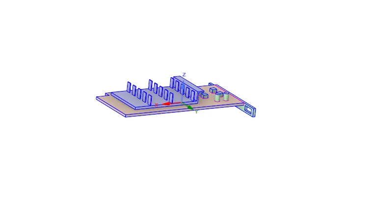
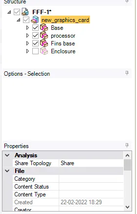
Now that we setup the geometry with share topology we are going to mesh and as for base mesh we are going to go for less cell counts with
10mm element size.
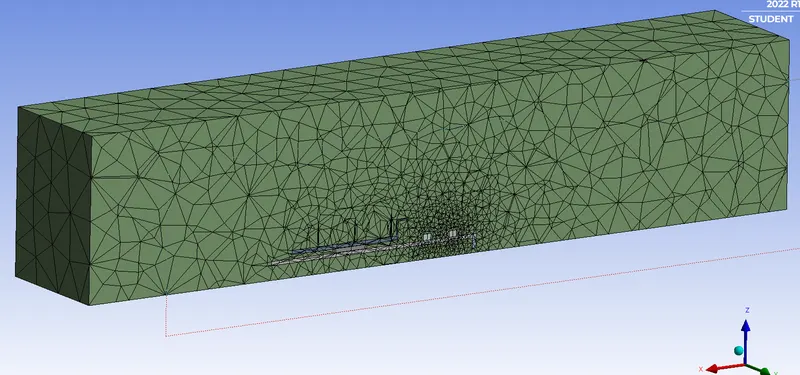
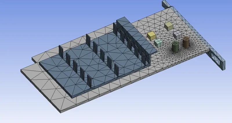
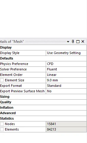
as we can see here we got ororsleves less number of element size of 84213 cell counts.
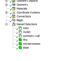
Now after naming the boundries we move onto Fluent for the simulation setup.
NOTE: that we ran k-omega SST viscous model for base mesh for little bit of variation in cases.
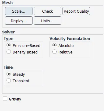
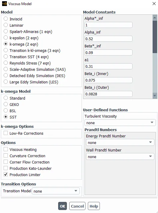
We can see the components in display where we visualize each and every art and interiors for the clearance and confirmation.
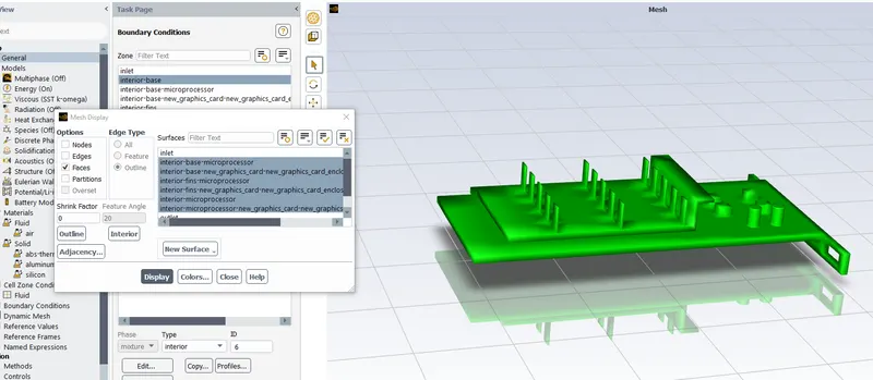
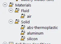
we have created and added 3 solids and 1 fluid for the geometry
Silicon - Microprocessor
ABS Thermoplastics - Base
Aluminium - Fins.
Fluid - Air
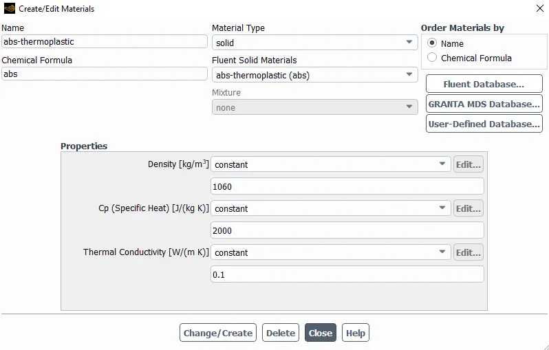
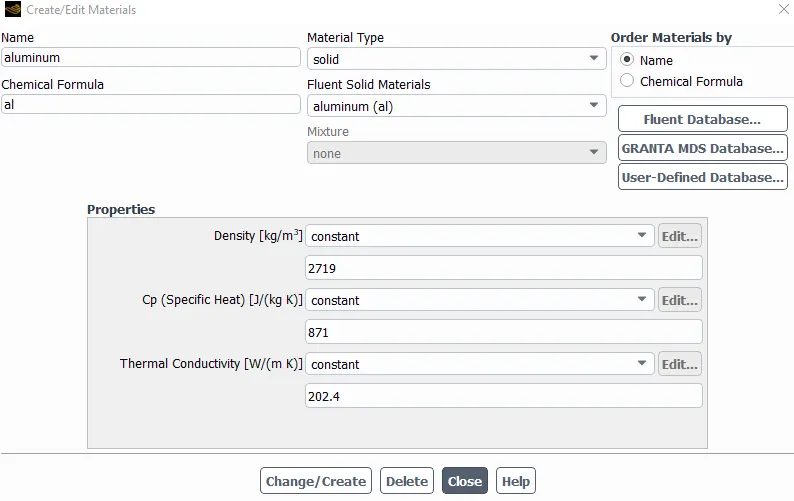
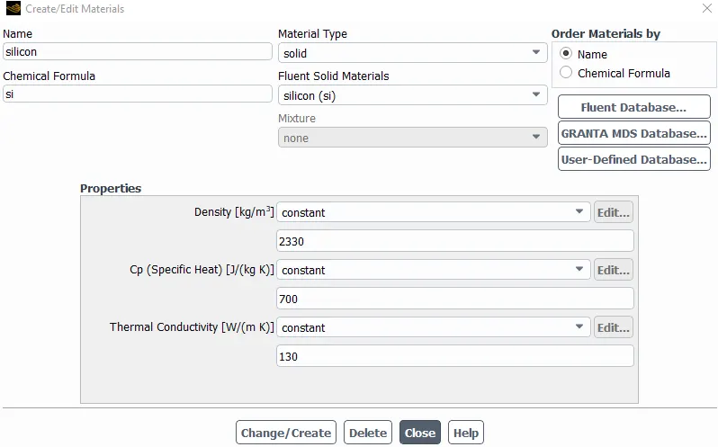
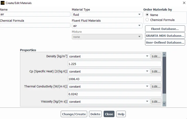
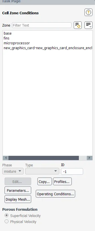
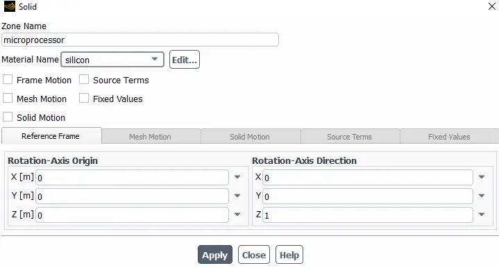
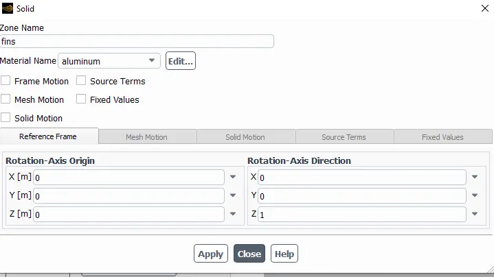
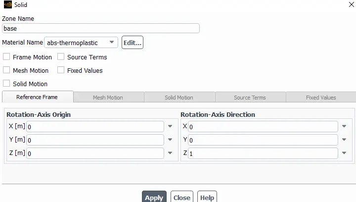
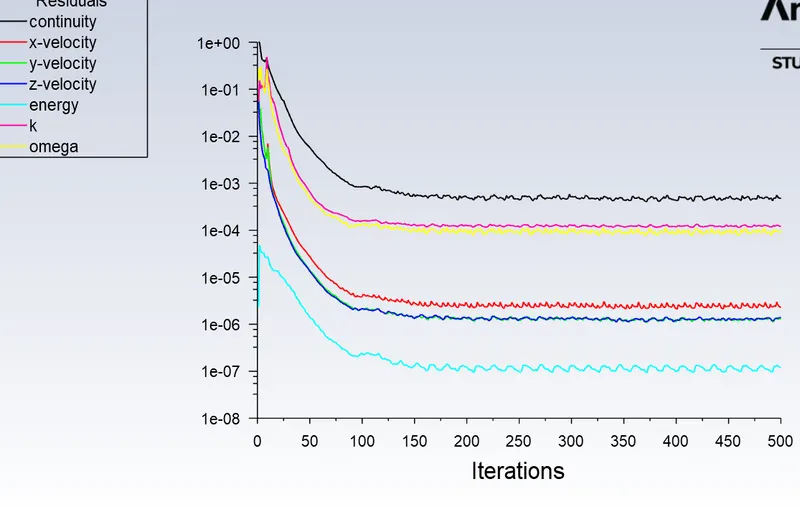
and he after setting up th materials and assigning the fluid and solid zones separately we run for 500 iterations and see that the solution is converged.
Output:
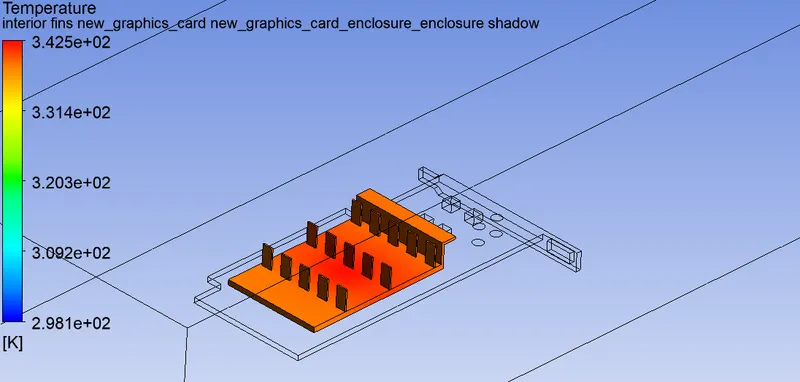
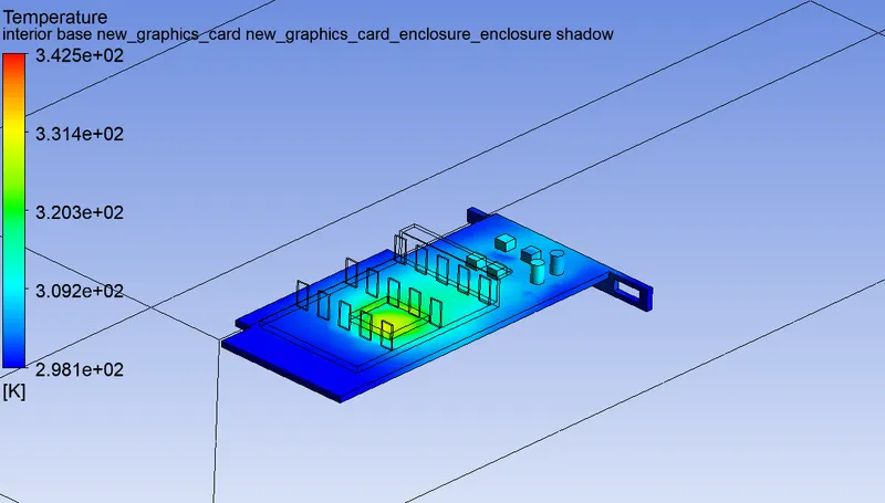
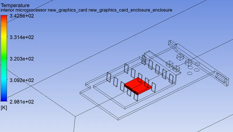
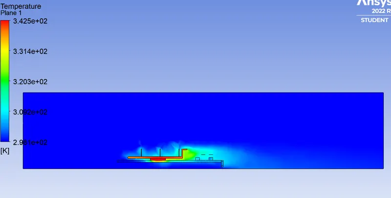
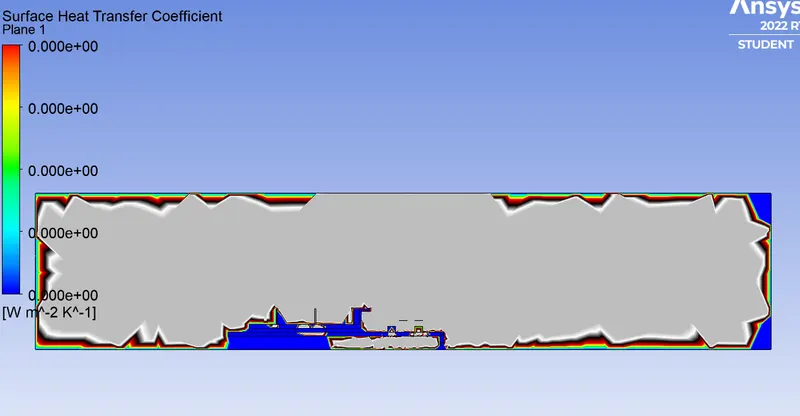
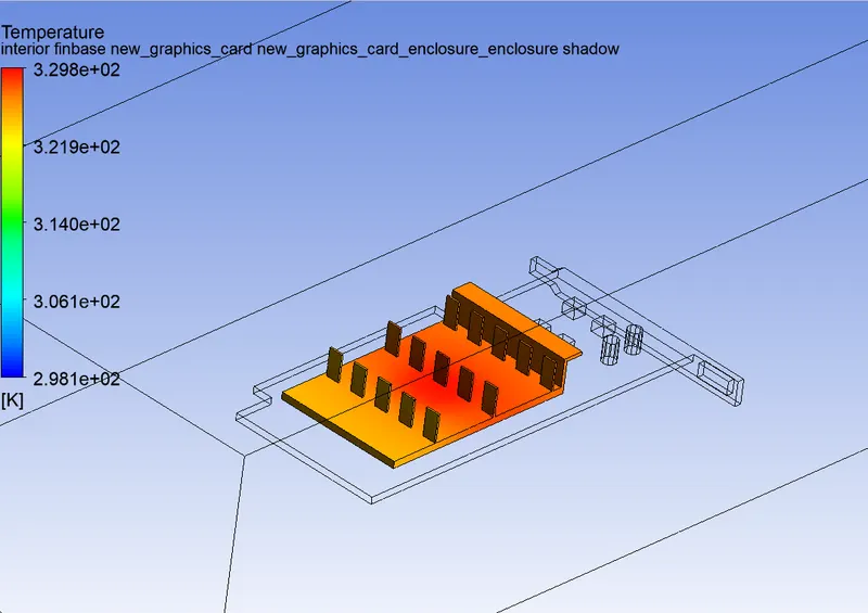
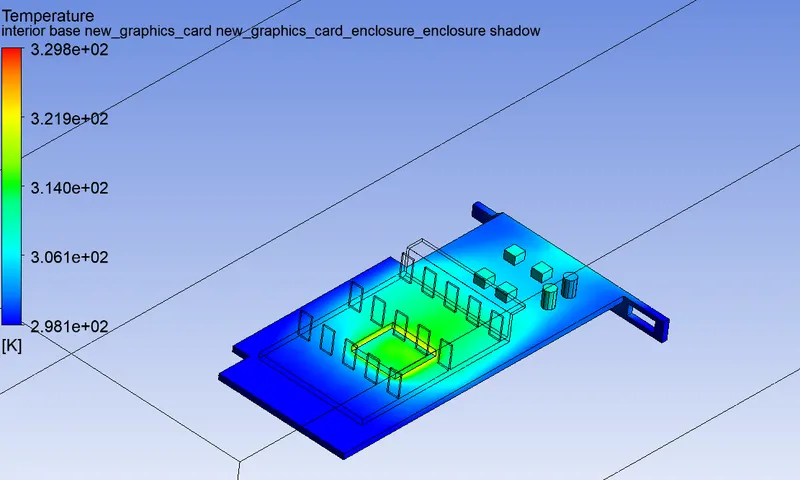
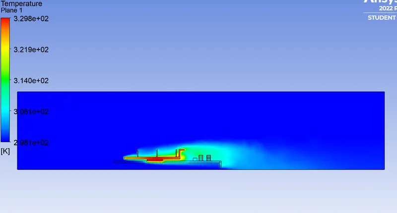
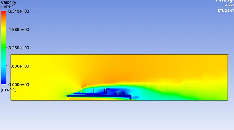
Now we are going to analyze the result in CFD-Post here we discuss the variation of temperature and velocity over the components and how heat transfer takes place.
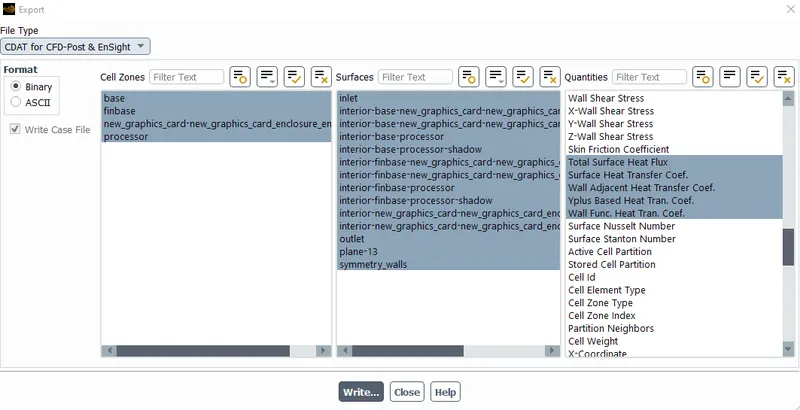
we take solution DATA and export it to CFD-Post via this method:
Temperature:
Velocity:
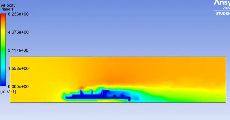
Heat Transfer Coefficient:
CASE 2: Refined Mesh
Now here we have refined the setup and made it to 499700 cells just near the academic license limit. The finer mesh will let us give precise results around the edges and the heat transfer coefficient. This is what we made the mesh accordingly:
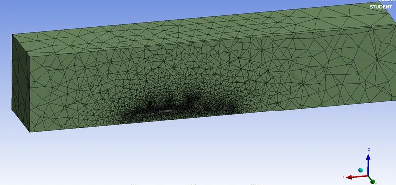
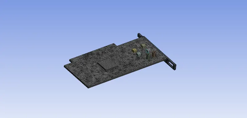
As you can see here when the element size is reduced the mesh gets finer and more importantly around the microprocessor and the base components, the mesh is structured by itself as we apply body sizing mesh tool to MICROPROCESSORS and FINS.
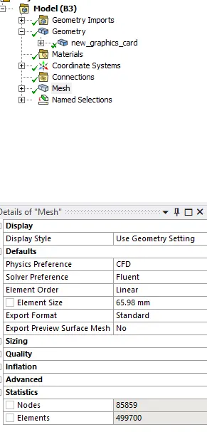
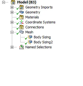
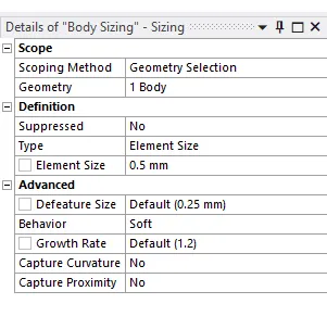
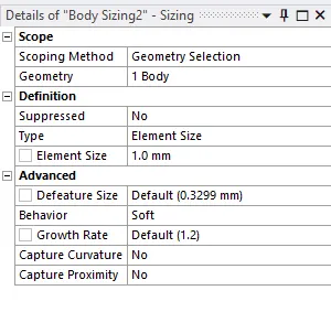
The main reason why we went for refining and specifically the kind of refining where we select the body and sized it down to 0.5 and 0.1 mm element size respectively.
Choosing the Refined mesh settings:
We are more interested in the thermal energy transfer from Microprocessor to Aluminium fin where it cools with airflow and this is where our turbulence model also plays a vital role, well there's not much of difference in its varietals, but this tells us how heat transfer takes place and this is the only 2 body in the GPU where the temperature is at highest, and we can see that in out BASE MESH fin and microprocessor CFD-post results.
That's why we refine these 2 whole bodies alone where we can exact results in simulation. In Base mesh, the results may not be viewed accurately as the mesh is too coarse not only around 2 Hotspot bodies but the GPU as a whole.
Now that we did setting up the mesh we move on to Fluent where we set up the geometry the same as BASE MESH with one difference where we use K-Epsilon Viscous model for the refined case just to make a variation in results and to play with the turbulence model.
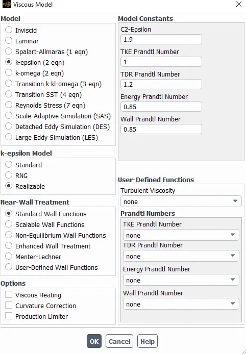
And now we INITIALIZE and run for 500 iterations where we see converged results.
Output:
Residuals where the solution is converged:
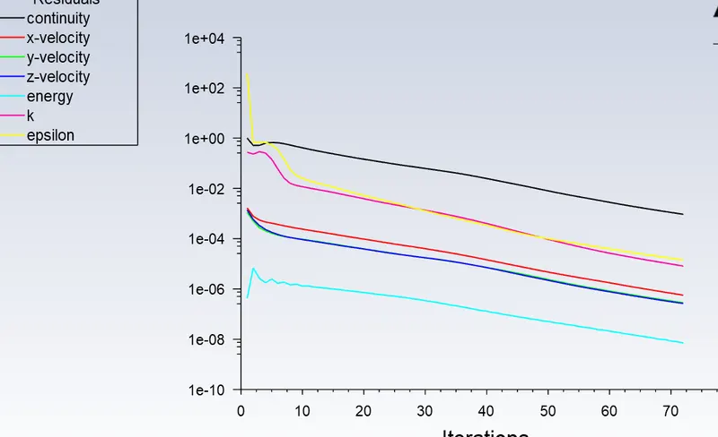
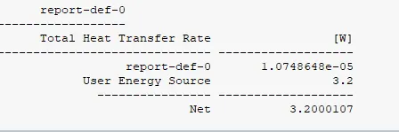
Now we export results as solutionDATA to CFD-Post where we analyze the results more clearly
Temperature:
Velocity:
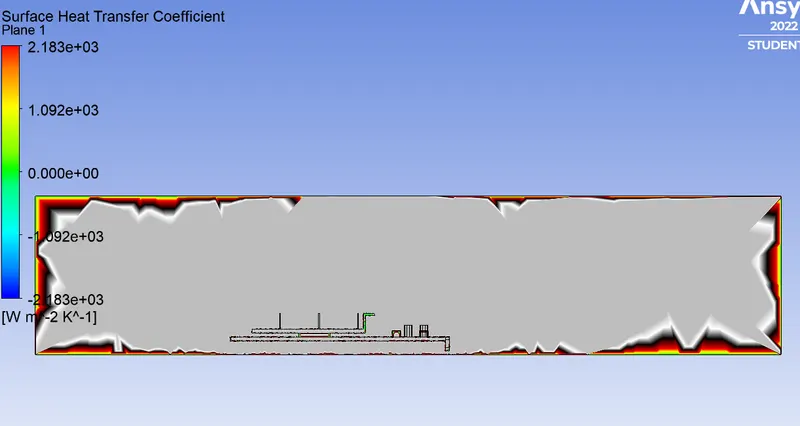
Heat Transfer coefficient:
Mains:
1. Run the simulation by varying the velocity from 1m/sec to 5m/sec for at least 3 velocities and discuss the results.
since it has 3 cases we gonna divide this into 3 sections where we study and analyze the temperature and HTC difference in different cases.
case 1: where Velocity is 1ms-1
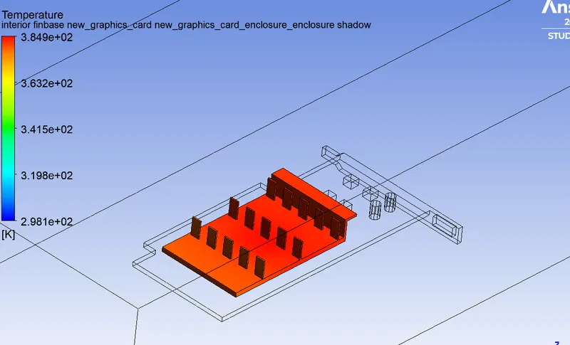
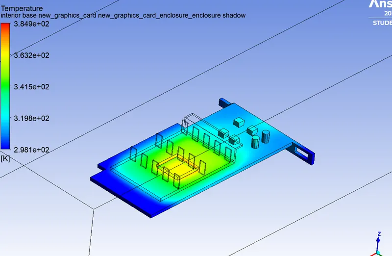
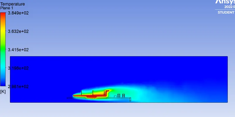
Temperature:
Velocity:
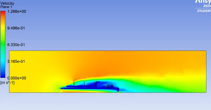
As we can see in our results the velocity varies around the edges reaching up to 12.66ms-1
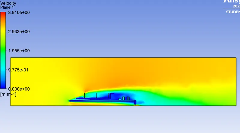
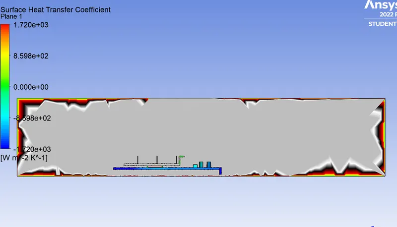
case 2: where Velocity is 3ms-1
Temperature:
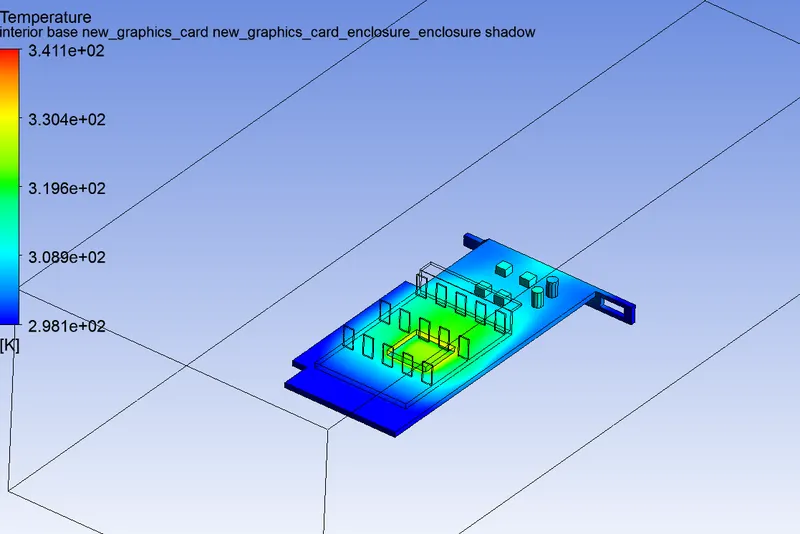
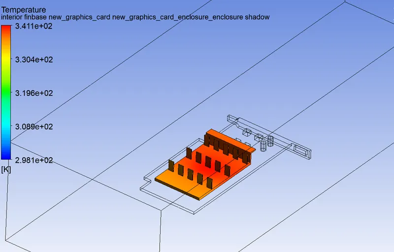
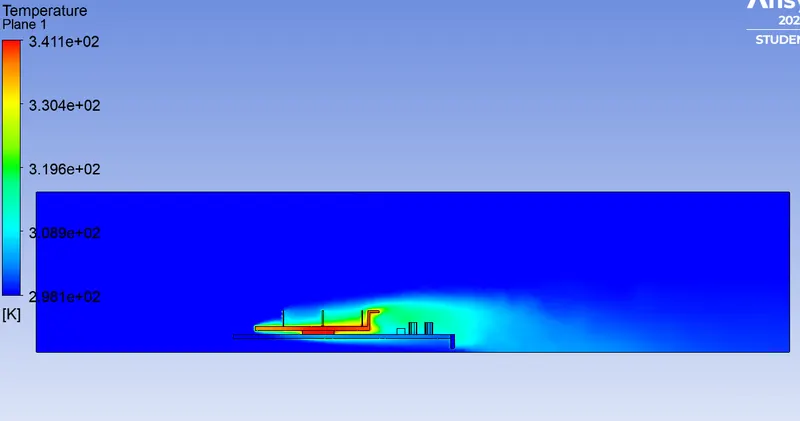
Velocity:
HTC:
case 3: where Velocity is 5ms-1
Velocity:
Heat Transfer coefficient:
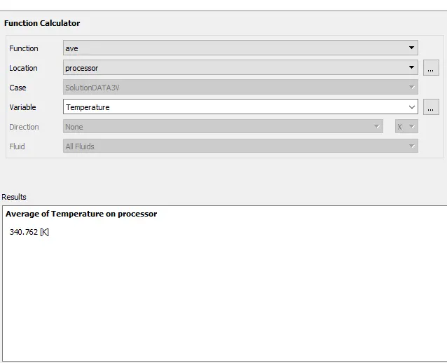
2. Find out the maximum temperature and heat transfer coefficient attained by the processor.
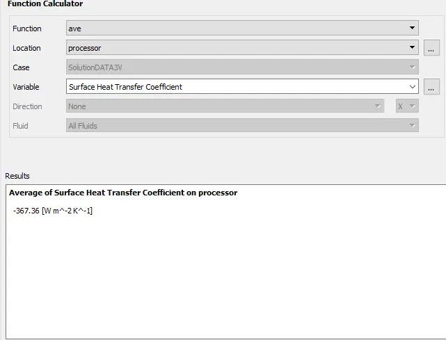
as we can calculate analytically with the plot and solution data but in CFD-Post we have special features to calculate the different functional areas and their averages so this is where we calculated results:
The following are calculated in refined setup case:
Heat Transfer Coefficient:
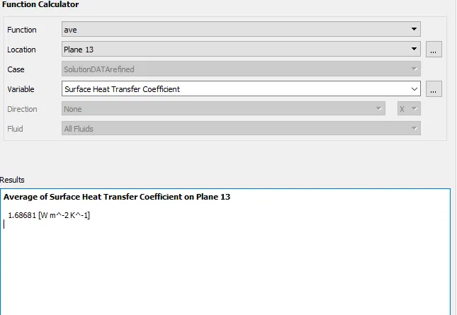
This is when we rin the cases for Velocity as 1ms-1 and 3ms-1 respectively by the Processor.
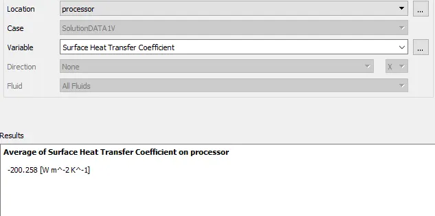
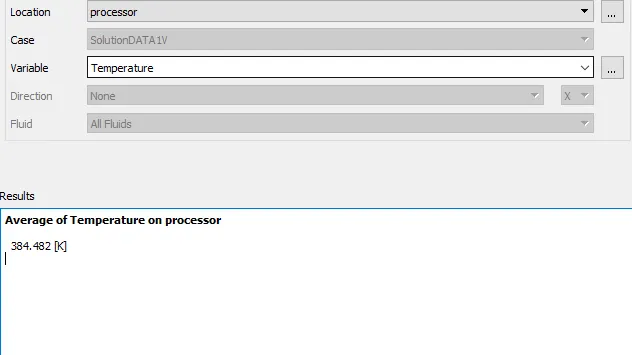
Case 3ms-1
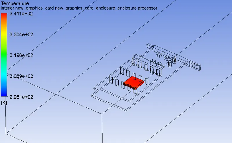
Max temps by the processor is 340K
3. Prove that the simulation has achieved convergence with appropriate images and plots.
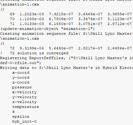
Here we can see that at 72nd Iterations the solver says that the solution is converged. And we can confirm this by looking at Residual Plots.
Refined setup:
Base Mesh setup:
4. Identify potential hotspots on the model.
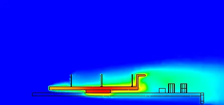
For identifying the Hotspots we have studied and analyzed several cases for the temperature and HEAT transfer coefficient.
so we know that the most potential Hotspots are around the Fin base and the whole microprocessor.
References:
Conjugate Heat Transfer Simulation: Best Practices | SimScale