Week-6 Calculate the Stretch Ratio by comparing the ELFORM (-2,-1,1,2) with Ogden_Material Model.
Aim:
To compare various ELFORMS against the Uniaxial Plot given and the Stress/strain developed in the uniaxial tension test
Explanation:
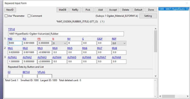
The given material card is opened into the LS PrePost application.
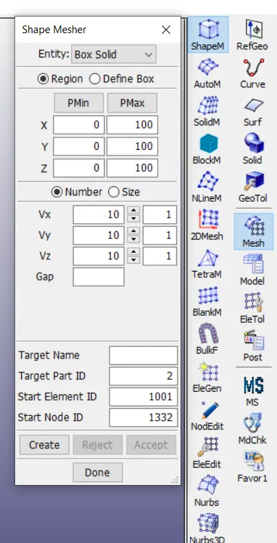
To develop Solid Cube mesh, go to
Mesh -> ShapeMesh -> Provide values such that a cube of 10x10x10 is developed with 10 elements on each direction
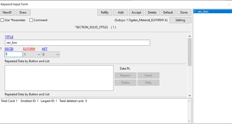
we will create section card for the solid with ELFORM 1,-1,2,-2
Model -> Keyword -> Section -> Solid
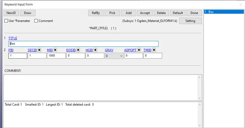
Now we will assign the section and material to the part
Model -> Keyword -> Part
Now we will develop boundary conditions to simulate the uniaxial tension test
we will first create nodesets for constraints and prescribed motion set.
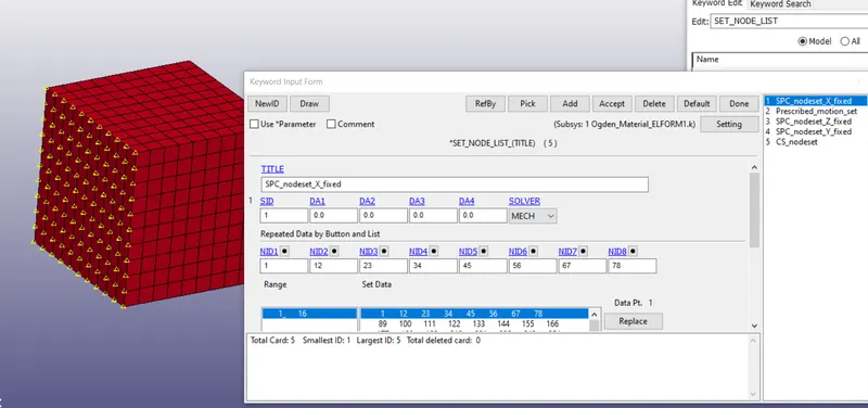
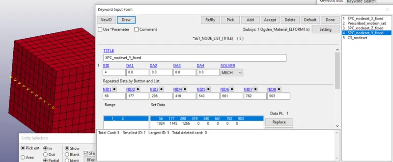
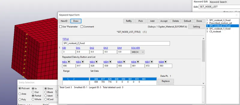
To simulate real behaviour of the material under uniaxial tension test, the constraints should be as described in the figure.
Nodes with X translation and all rotation constrained
Nodes with Y translation constrained
Nodes with Z translation constrained
Nodes for Prescribed Motion Set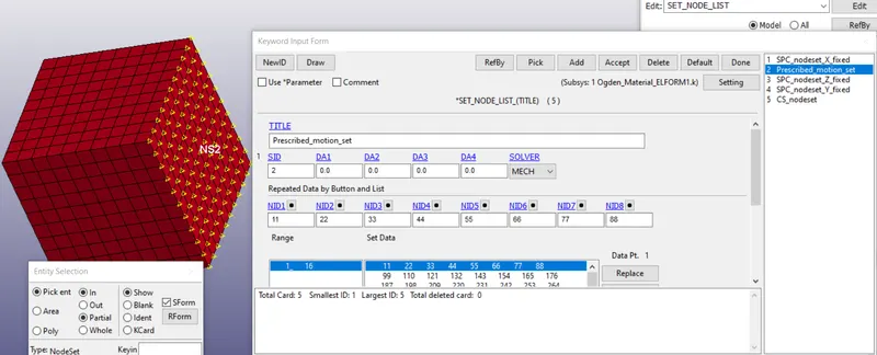
Using Boundary -> SPC set and Prescribed motion set, we can develop the boundary conditions as described.
A curve can also be used for the Precribed motion set card
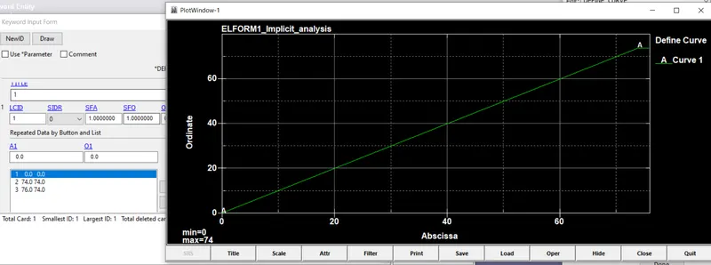
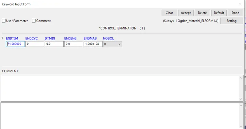
We will use termation time for simulation as 74ms to have enough points to plot Stretch/Strain Vs Stretch ratio upto 5
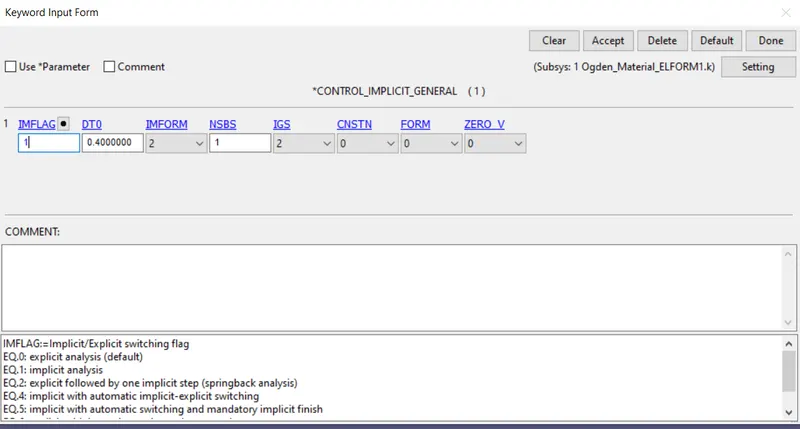
We will use Implicit Analysis for the uniaxial tension test as it a quasi static process and since we are only concerned with the end state of the simulation, Implicit analysis will be more faster
Its always a best practise to use the following 4 cards under Control keyword while using Implicit Solver
- Implicit General
- Implicit Auto
- Implicit Solution
- Implicit Solver
Implicit General: Used to Invoke Implicit Solver (IMFLAG) and to specify starting time interval (DT0)
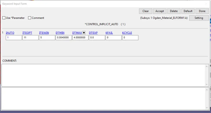
Implicit Auto: Used to dynamically change time interval using ITEOPT and ITEWIN. If the number of iterations in a step is between (ITEOPT-ITEWIN) and (ITEOPT+ITEWIN), there wont be any change in DT. If it lesser, DT will be increased. If it is more, DT will be reduced. Also need to specify how small and how large DT can be under DTMIN and DTMAX during the process.
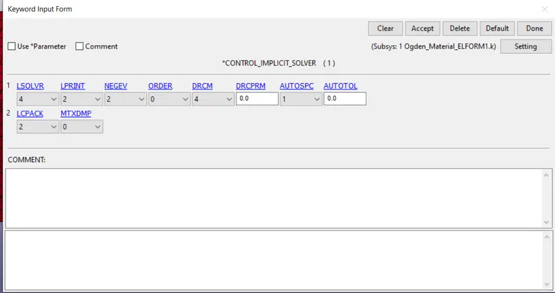
Implicit Solver: Controls Linear part of the solution. Usually LSOLVR and LCPACK are the ones changed
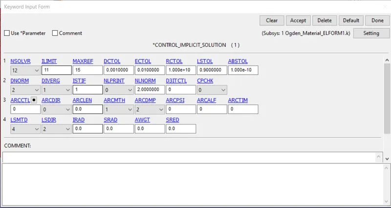
Implicit Solution: Non Linear part of the Implicit Solver. ILIMIT, MAXREF, DCTOL, DNORM are the ones usually changed. Controls Stiffness matrix reformation times and Displacement Tolerance (DCTOL)
Binary D3Plot can be invoked under
Model -> Keyword -> Database -> Binary_D3Plot with 0.5ms dt
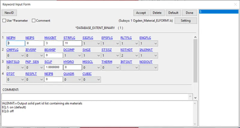
We need to add
Database -> Extent_Binary and activate STRFLG to get strain data.
Now the model is built and can be run.
POST PROCESSESSING:
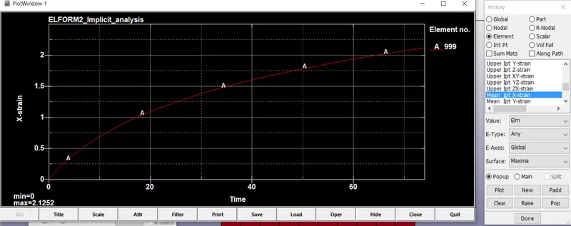
Now plot the IPT X strain and Effective Stress from
History -> Elemental -> select an element -> IPT X strain / Effective Stress
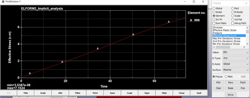
Save the curves
Now do cross plot with these 2 curves
XY Plot -> Cross plot -> select appropriate curves to plot stress vs strain
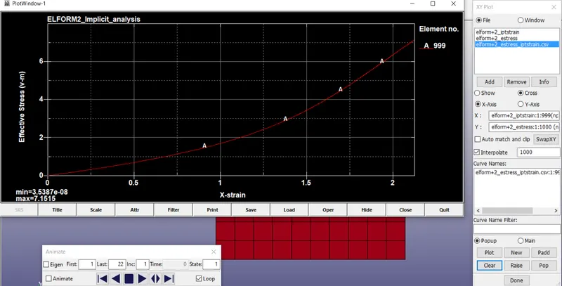
Save the curve in CSV format. Do these for all ELFORMS -2,-1,1,2
open the excel file and add columns for Stretch ratio and Engineering stress
Stretch ratio = e^(true stress)
Engineering stress = True stress/stretch ratio
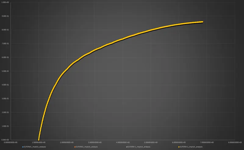
All the ELFORMs are plotted and all follow the same path
Conclusion:
The plot shows that Stress Vs Stretch ratio is not affected by the type of these Element formulations
EQ.-2: fully integrated S/R solid intended for elements with poor aspect ratio, accurate formulation.
EQ.-1: fully integrated S/R solid intended for elements with poor aspect ratio, efficient formulation.
EQ.1: constant stress solid element (default),
EQ.2: fully integrated S/R solid
and all the curves follow the same path. The stress increases initially, reaches a maximum point and then decreases. The point where the stress starts to decrease in value is called the Necking point. Once necking point is reached, the solid elongates easily without much effort, and hence the stress decreases.