Week-6 Calculate the Stretch Ratio by comparing the ELFORM (-2,-1,1,2) with Ogden_Material Model.

Objective: Perform Volumetric Tensile test on a Odgen(Rubber) material cube by using appropriate boundary conditions with different element formulation of solid (1, -1, 2,-2) and compare results upto Stretch ratio of 5.

1. Create a block of 10mmx10mmx10mm dimension with 10 elements for each direction and use the material card attached (Ogden_Material.k) that is representative of the material properties from the above figure.
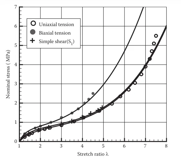
2. Use appropriate boundary conditions to simulate tensile behavior for the model and finally compare the results from your simulation to the plot above up to stretch ratio 5. Only the uniaxial plot is to be compared.
3. Compare the results for the simulation using ELFORM = 1, 2, -1, -2
4. The unit of µ in the material definition is in MPa and α is a dimensionless quantity. Modify those quantities according to your unit systems.
5. Use a proper solver (Implicit/Explicit) and also explain the reason.

Procedure:

Modelling:

Model a cube with 10mmx10mmx10mm dimension with 10 elements for each direction by going to Mesh panel> Shape mesher> Enter values for creating Box> Apply> Done.

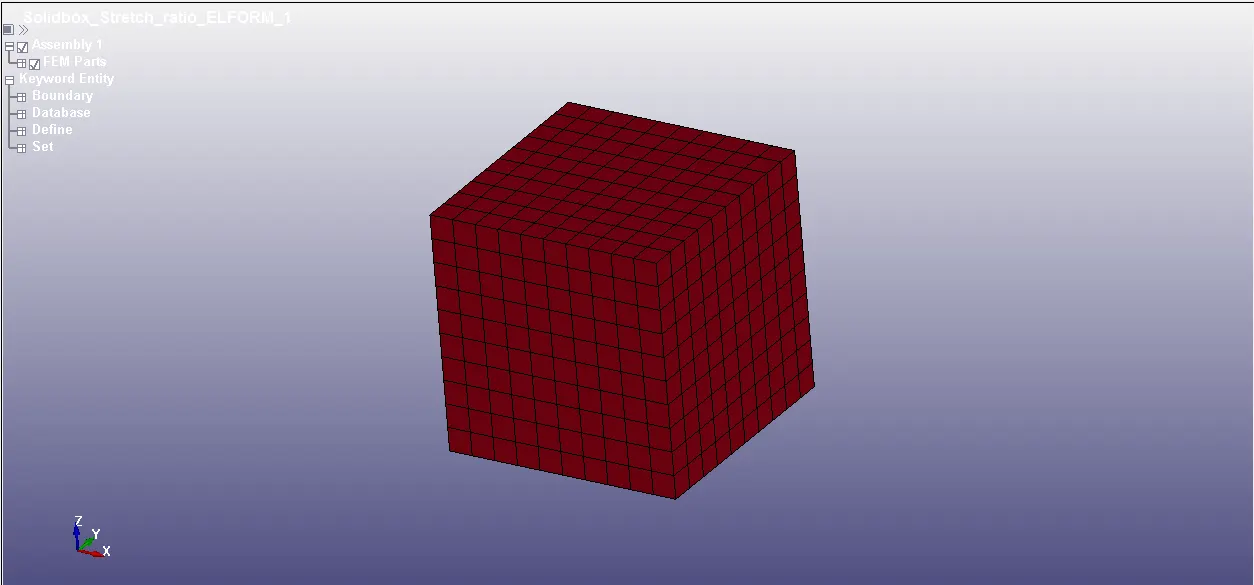
Created Box with required dimensions

Section:

Since Elements are Solid and we need to compare with different Element formulation (1,-1,2,-2) so only one Section card is shown.

ELFORM=1 : Constant stress solid element . Default

ELFORM=-1 : Fully integrated S/R solid intended for elements with poor aspect ratio , efficient formulation.

ELFORM=2 : Fully integrated S/R solid

ELFORM=-2 : Fully integrated S/R solid intended for elements with poor aspect ratio , accurate formulation.

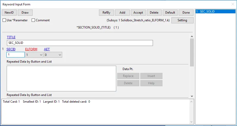
Section card of ELFORM=1

Material:

A material card MAT_ODGEN_RUBBER is created which is an Hyperelastic material and the values are taken from the given (MAT_ODGEN.K) card.

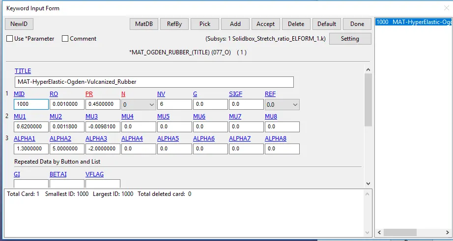
Material card for Box

Part:

Section and Material are assigned in the part card with the help of their ID.

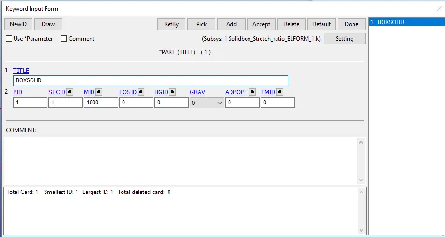
SECID and MID are assigned in Part card

Boundary conditions:

Boundary_SPC

Since we are performing a simple tensile test so we have to constrained one side and apply motion on other side. As it is a solid box so we are providing Three Boundary SPC on one face of box . On one face , All nodes are constrained on Translational X- direction with Rotational constrained provided in all the directions . Mid nodes of same face are selected Constaining Translational Y along Z-direction and Constraining Translational Z along Y- direction.

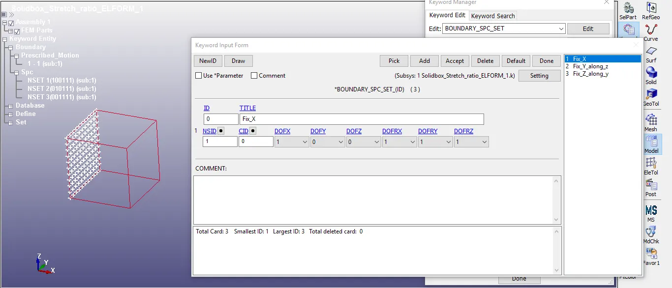
Constraining one face along X and all rotational directions

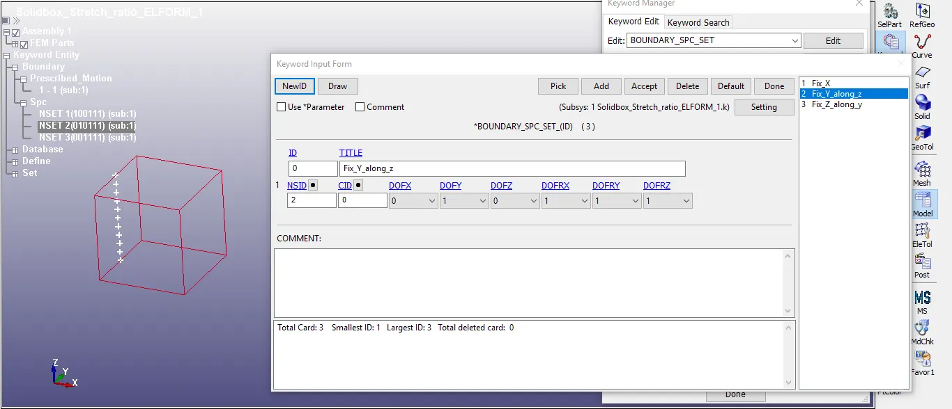
Constraining mid nodes lying on Z along Y direction

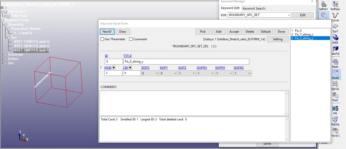
Constraining mid nodes lying on Y along Z direction

Prescribed Motion

In order to impose any kind of load Boundary_Prescribed_Motion_Set is card. As it is an Implicit , so instead of load an imposed displacement will be given to the set of nodes lying exactly opposite to the face of constraining. As we need to plot graphs upto Stretch ratio of 5 , so we need to calculate minimum displacement required for the test.

Stretch ratio `lambda=1+epsilon_e` where `epsilon_e` is the Engineering strain`=(deltal)/l`. Therefore , we need to find `(deltal)` for which Stretch ratio, `lamda=5``=>5=1+(deltal)/10=>deltal=40mm`. Thus we will need our displacement curve by giving displacement value of 60 mm.

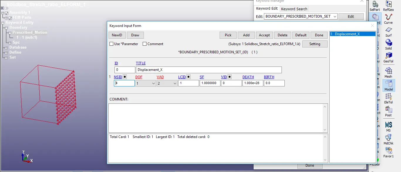
Prescribed motion set card

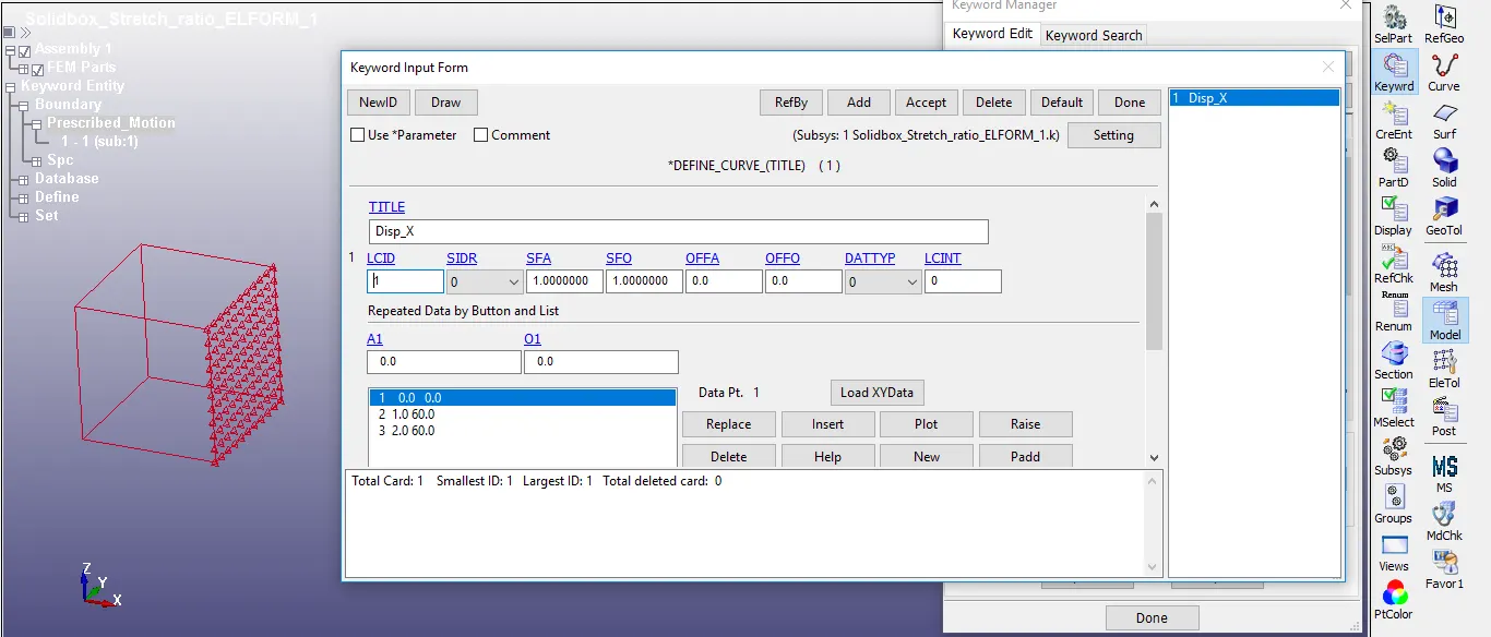
Displacement Curve card

Reason for choosing Implicit solver over Explicit:

The model is a Non-Linear Implicit Quasi Static Analysis the reasons are as follows

• Here, in this model the material used is Ogden (vulcanized rubber) which is a Hyperelastic material, which undergoes Nonlinear deformations.The material Nonlinearity is the reason why the model is considered to be Nonlinear (solid (hex) -1, 2, -2)
• The implicit methods are used when the effects of strain rates are very minimal. The explicit methods are used when the strain rates/velocity are over 10m/s. In Implicit method the displacement loading is recommended rather than Force load to achieve more stable load.
• Quasi Static: 'Time' represents a monotonically increasing parameter which characterizes the evolution of loading but here the load is replaced with displacement.

Control cards:

To perform an Implicit Analysis, it is a must that the CONTROL_IMPLICIT_GENERAL is called for. This keyword makes sure that the analysis is solved in Implicit method. The IMFLAG is set to 1, so that, it enables the method to switch from Explicit to Implicit as Explicit method is default in LS-DYNA. DTO is set to 0.01.

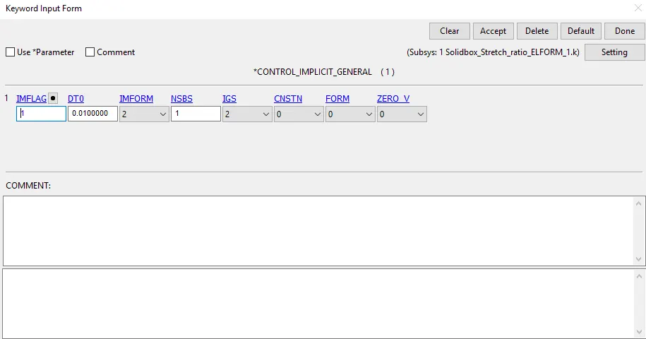
Control Implicit General Card

CONTROL_IMPLICIT_AUTO: The purpose of this keyword is to maintain automatic timestep. (AUTO is set to 1 which automatically adjusts the timestep size. ITEOPT optimizes the operation count step. ITEWIN is the iteration window. DTMIN is DT/1000 and DTMAX is DT*10.

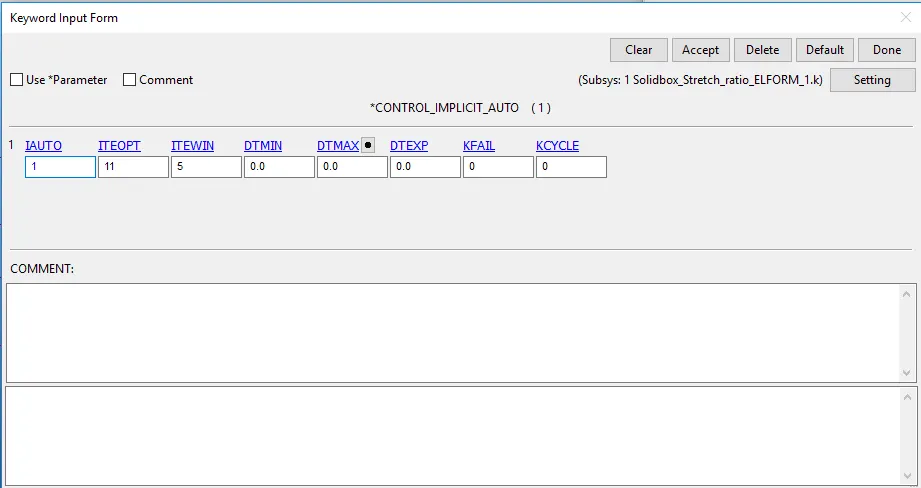
Control Implicit Auto Card

CONTROL_IMPLICIT_SOLUTION: This card is used to choose between linear and nonlinear analysis in implicit method. NSOLVR is set to 12 by default and LSMTD which is a Line Search Convergence Method is by default set to 4.

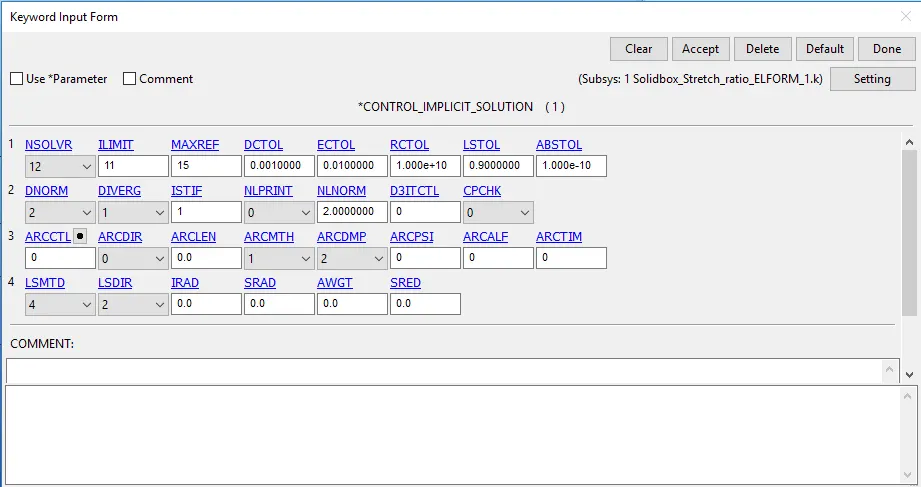
Control Implicit Solution Card

CONTROL_IMPLICIT_SOLVER: The stiffness matrix inversion is being done through this keyword. LSOLVR is by default set to 2 which is a single precision solver, but it is advisable to use 5 which is a double precision solver for better results in case of a complex implicit analysis.

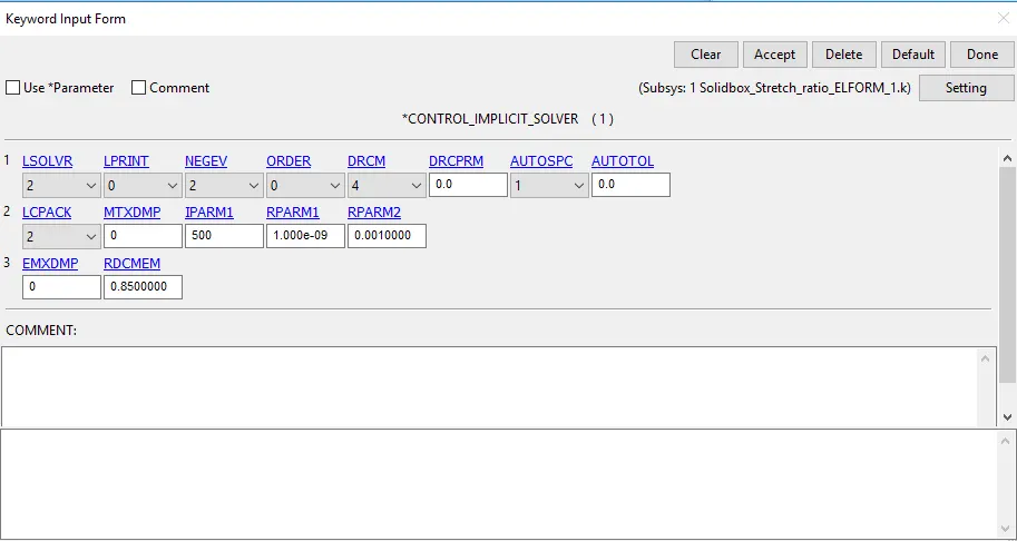
Control Implicit Solver Card

CONTROL_TERMINATON: End time of simulation is given as 1 ms.

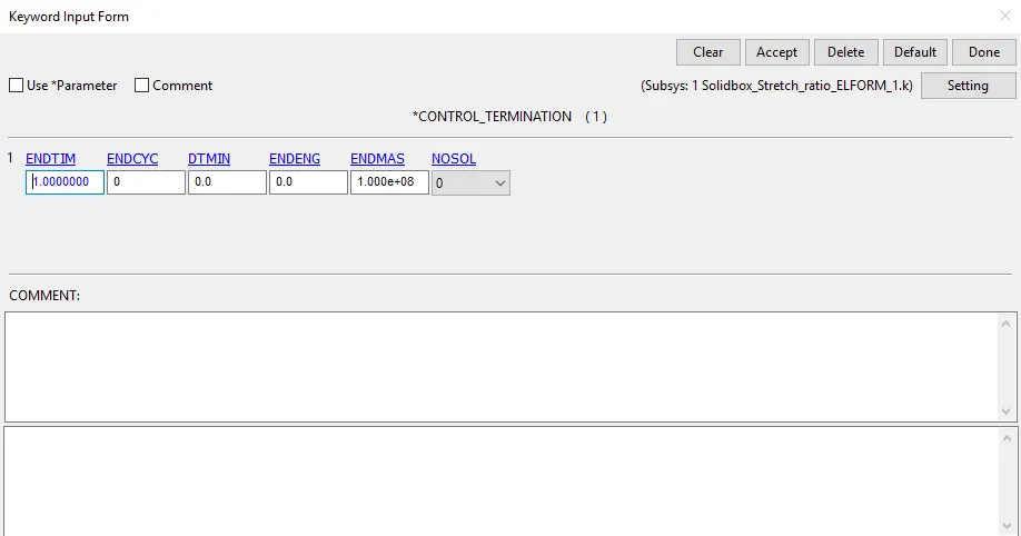
Control Termination card

Output Requests:

Database binary D3PLOT is created to get the animation of simulation. DT=0.1 ms

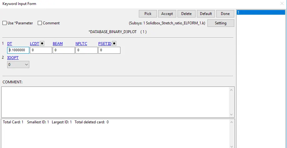
Binary D3PLOT card

Database Extend Binary is created to get data related with stress and strain obatined frm the animation. STRFLAG is kept as 1 and rest are kept as defaults.

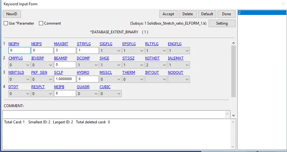
Database Extend Binary card

Database History Solid card is created to get values from a Solid element. In our case Element ID 550 is selected as it lies in middle of the box.

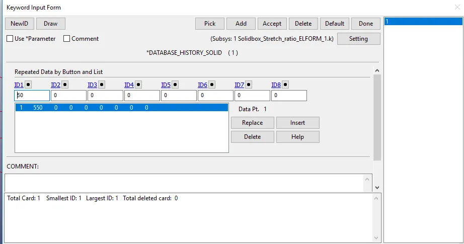
Database History Solid card

Post processing:

Open the keyword file and the d3plot file in LSPP. Play the animation to visualize the results of the applied boundary conditions. Generate the stress and strain contour animations. Now we need to select one element and use the History option to plot the x-stress and x-strain for that element. In this case, element number 550 is selected which is approximately at the center of the box. Save the plot details as an excel file. The stress and strain values recorded in LS Dyna are true stress-strain values. We are asked to plot the Engineering Stress vs stretch ratio for the four cases. We need to calculate the Engineering stress-strain values from the true stress-strain values taken from the LS Dyna plots as shown below:

We know, True stress `bbsigma_(true)=bbsigma_(engg)*(1+bbepsilon_(engg))=>bbsigma_(engg)= bbsigma_(true)/(1+bbepsilon_(engg)`

Similarly , True strain `bbepsilon_(true)= ln(1+bbepsilon_(engg))=>bbepsilon_(engg)= e^(bbepsilon_(true))-1`

By using above equation we calculate Engineering stress and strain and tabulate the results. We have evaluated Stretch ratio as well `bblamda = 1+bbepsilon_(engg)`

Animations of simulation:

X-stress and X-strain for ELFORM=1

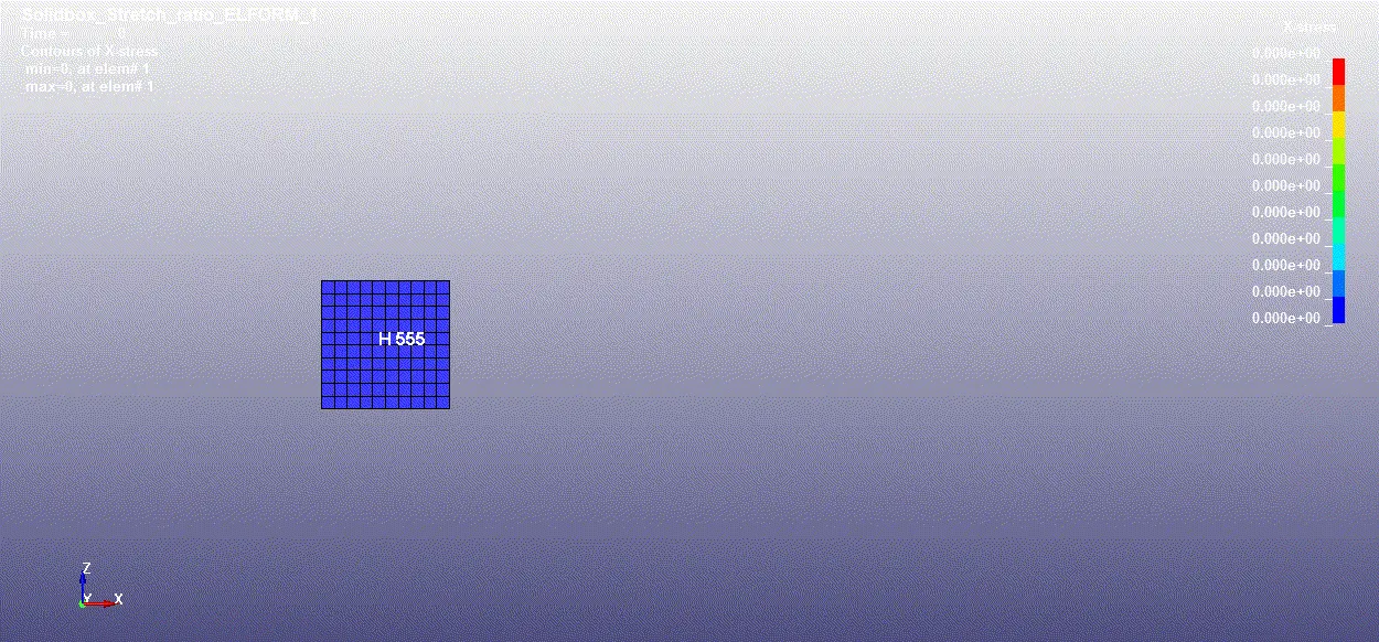
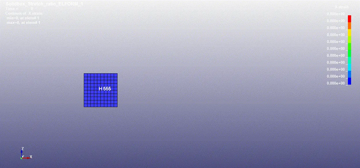
The maximum X-stress and X-strain obtained in ELFORM=1 is 6.00914 MPa and 1.94288 respectively.

X-stress and X-strain for ELFORM=-1

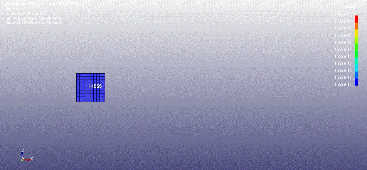
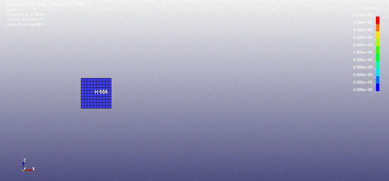
The maximum X-stress and X-strain obtained in ELFORM=-1 is 5.99997 MPa and 1.941 respectively.

X-stress and X-strain for ELFORM=2

The maximum X-stress and X-strain obtained in ELFORM=2 is 5.99801 MPa and 1.90058 respectively.

X-stress and X-strain for ELFORM=-2

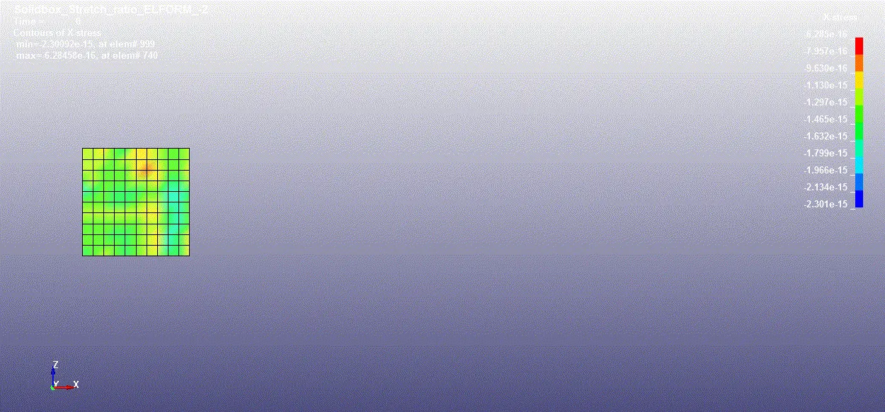
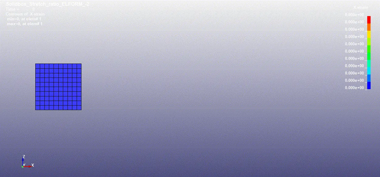
The maximum X-stress and X-strain obtained in ELFORM=-2 is 5.99651 MPa and 1.94087 respectively.

Table with data

ELFORM	X-STRESS MPA	X-STRAIN
1	6.00914	1.94288
-1	5.99997	1.941
2	5.99801	1.90058
-2	5.99651	1.94087

The tension test was simulated for a cubical box modeled with Hexa elements and hlyperelastic Ogden material model

After comparing from above table , we can see that ELFORM=1 gives maximum value of X-stress and X-strain.

Comparing datas for upto Stretch ratio 5 with provided material curve:

Since our area of interest is upto Stretch ratio of 5 , so below are the tables of different ELFORM used and are compared with each other with proper material curve provided to us. This is provided material curve . We have compare our different cases for upto Stretch ratio of 5.

ELFORM=-1

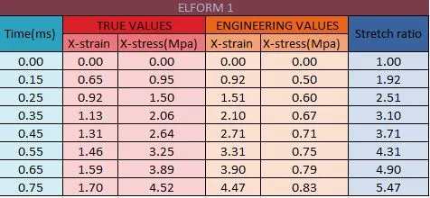
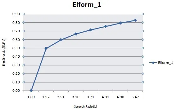
For approximate Stretch ratio 5 , we are taking Stretch ratio of 5.47 for which Engineering strain and stress is 4.47 and 0.83 MPa.

ELFORM=-1

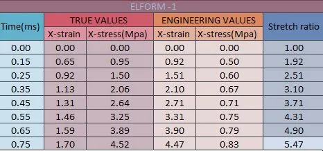
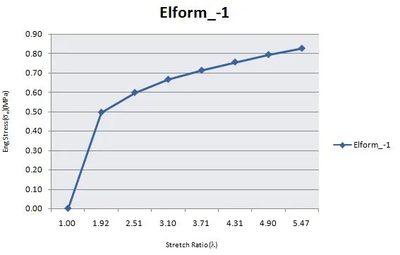
For approximate Stretch ratio 5 , we are taking Stretch ratio of 5.47 for which Engineering strain and stress is 4.47 and 0.83 MPa.

ELFORM=2

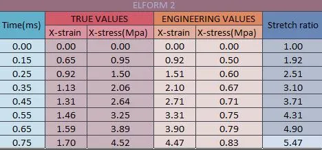
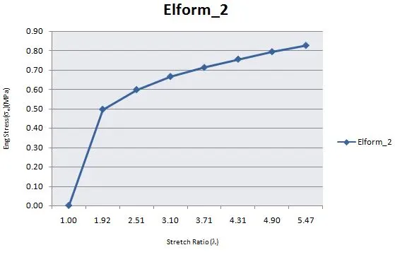
For approximate Stretch ratio 5 , we are taking Stretch ratio of 5.47 for which Engineering strain and stress is 4.47 and 0.83 MPa.

ELFORM=-2

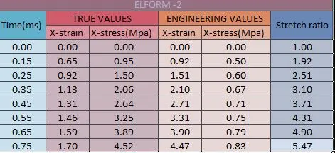
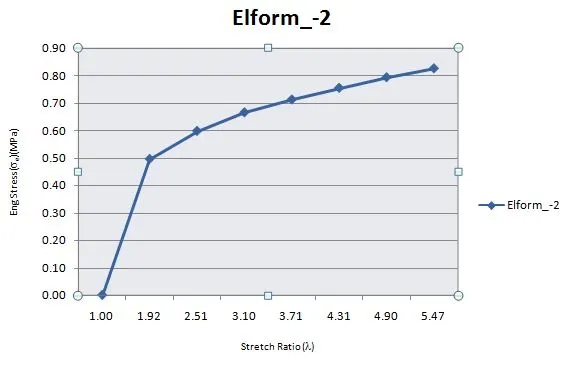
For approximate Stretch ratio 5 , we are taking Stretch ratio of 5.47 for which Engineering strain and stress is 4.47 and 0.83 MPa.

The curves for all the cases are nearly the same with the Engineering stress value recorded to be —0.83 MPa for a stretch ratio of 5. On comparing the curves plotted with the original curve for the material model, we see that not much stress has been induced on the elements. The original curve shows stress of —1.6 MPa corresponding to a stretch ratio of 5, whereas the plots we have generated only show —0.83 MPa for the same stretch ratio. If we compare the shape of the original curve and the generated ones, we can also see that the shape of the curves is similar up to a stress of 0.83 MPa but the difference is that 0.83 MPa stress in the original curve corresponds to a stretch ratio of 2 compared to 5 in the generated curves. This difference could be due to the fact that we have not followed the tension test standards correctly. In a proper tension test, the specimen has to be of a particular size and everything is standardized. In our case, we have just used a random specimen and applied some arbitrary displacement. Thus the two results should not actually be compared.

Conclusion:

• The tension test was simulated for a cubical box modeled with Hexa elements and hlyperelastic Ogden material model. The test was performed with elforms 1, -1, 2, and -2.
• The true stress and strain values were used to calculate the engineering stress and strain values.
• The stretch ratio was calculated for all the cases and a plot of Engineering stress vs stretch ratio curves were created and compared.
• An implicit method was used to solve this tension problem as the rate of displacement imposed on the model was very low and thus, it was similar to a quasi-static analysis on a hyperelastic elastic non-linear material.