Week-6 Calculate the Stretch Ratio by comparing the ELFORM (-2,-1,1,2) with Ogden_Material Model.

Assignment 6

The objective of this assignment is to simulate 3 different load scenarios and compare them with the previous graph, considered as the Actual Data. In this comparison, 4 different element formulations will be used.

1. Block geometry

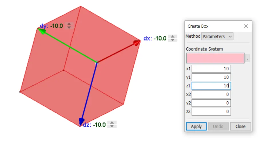
As requested for this assignment, the block must be 10x10x10 mm and have 10 elements in each direction.

First, a box was created with the indicated dimensions.

2. Block mesh

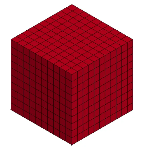
Using the solid mesher option, the required mesh was created

3. Section

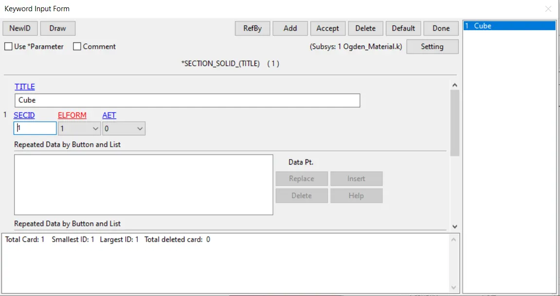
A section was created to associate the element formulation to the part:

4. Boundary condition setup

The next fluxogram displays the workflow of the next simulations:

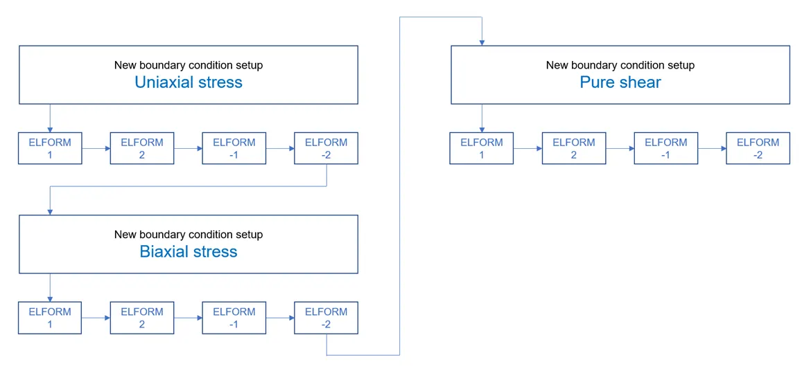
This means that, from the simulations that will be carried here, 12 groups of data will be extracted

4.1. Uniaxial stress

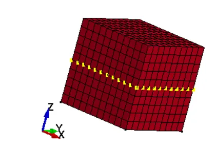
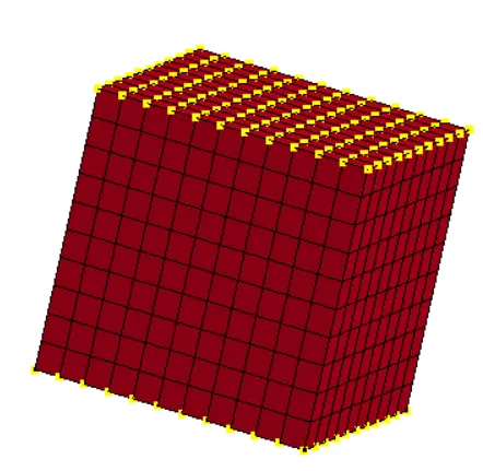
For this case, the nodes in the middle section (figure of the left) were prevented to move in the z direction. While the nodes on both surfaces (figure pof the right) were forced to move at a constant velocity and away from the middle section. A reasonable value for the velocity was thought to be 2mm/s (1mm/s for each extremity).

If we want to analyse the results until `\lambda`= 5, the final engineering strain value in the last instant of the simulation will be:

`\lambda = \epsi_e + 1 \Leftrightarrow 5 = \epsi_e + 1 \Leftrightarrow \epsi_e = 4 \Leftrightarrow \frac{L}{L_0} = 4 \Leftrightarrow \frac{L}{10} = 4 \Leftrightarrow L = 40 mm`.

This means that, in order for the cube to have a final height of 40 mm, each of the extrimities will have to travel 15 mm, as it is shown in the following figure:

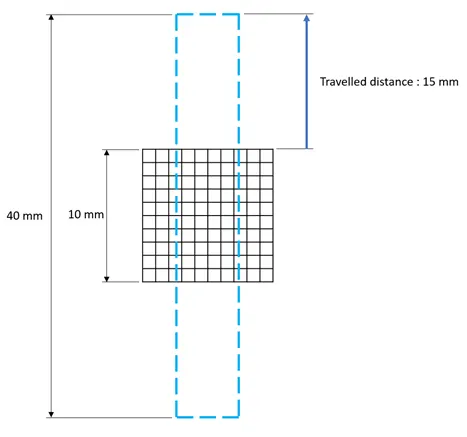
Knowing that the imposed velocity is 1 mm/s, we can calculate the total simulation time:

`\Deltat = \frac{\Deltad}{v} = \frac{15}{1} = 15 s`

Despite the calculated time is 15 s, the simulation time was set to 30 s because the results indicate that it is only at that that tim when the stretch ratio reaches the value of 5

5. Control keywords

Fot the uniaxial stress case, the total simulation time is large (30s), plus, the strain velocities are expected to be high (large deformations happening very quickly), therefore, an implicit solver will be used.

For this, two cards were created:

CONTROL_IMPLICIT_GENERAL

- Used to allow the software to vary between explicit and implicit solver, for the eventuality of being possible to achieve convergence in a less time consuming way.

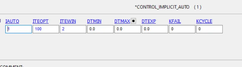
CONTROL_IMPLICIT_AUTO

- Restrictions applied to the number of iterations in each time step, to allow the time step to be increased. The value for ITEOPT and ITEWIN are 100 and 2 because, in principle, the total number of iterations in each time step is lower than ~100. And, if that is the case, the time step is increased

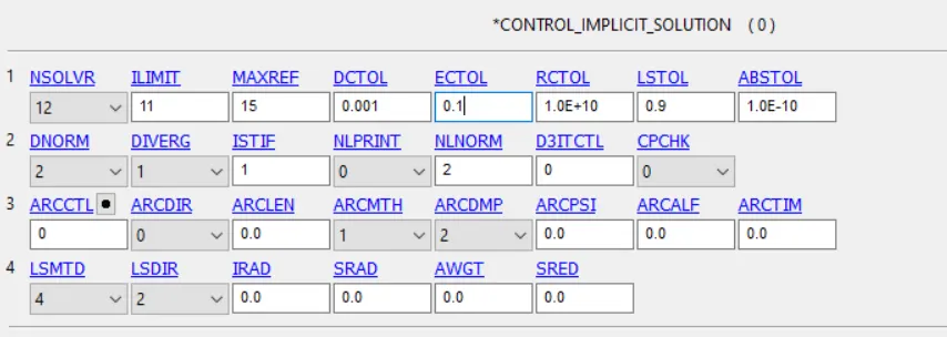
CONTROL_IMPLICIT_SOLUTION

This keyword is dedicated to the non-linear part of the calculations, and it is activated to define the tolerances for the residuals. The residual for the energy was changed to a less restrictive value so that the simulation can converge based only on the value of the residual of the displacement. The remaining parameters were left as default.

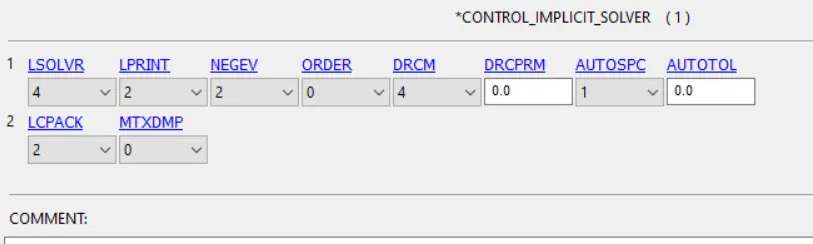
CONTROL_IMPLICIT_SOLVER

The linear part of the calculations is based in this keyword. All the values were left as default.

6. Outputs

The following keywords were activated to extract the desired outputs

DATABASE_D3PLOT

DATABASE_EXTENT_BINARY

7. Results

Due to complications with MS Excel, I resorted to MatLab to make a simple code to analyse the data.

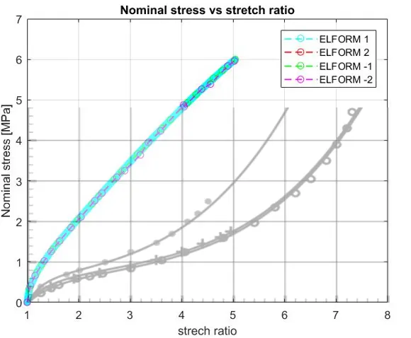
The following figure shows a comparison between the data extracted by using the 4 different element formulations and the given plot.

The results diverge significantly, meaning that some adjustments to the material paramenters need to be made to achieve a better match of the data.

8. Further conclusions

• In many occasions, the solver kept repeating the same error when the simulation was run. This problem was fixed by modifying the parameters ITEOPT and ITEWIN. By adjusting the number of iterations in each time step, the program overcame these errors and the results were extracted. The consequence of this manipulation is the difference of the time steps used for each element formulation: In the figure above, it is possible to see that the ELFORM 1 took much more time steps than ELFORM -2 to solve.
• This simulations could be improved if the nodes were prevented from rotating around the axis of the stretch direction, increasing the accuracy of the simulation