Rayleigh Taylor Instability

Rayleigh Taylor Instability

The Rayleigh–Taylor instability, or RT instability, is instability of an interface between two fluids of different densities which occurs when the lighter fluid is pushing the heavier fluid. Examples include the behavior of water suspended above oil in the gravity of Earth, mushroom clouds like those from volcanic eruptions and atmospheric nuclear explosions, supernova explosions in which expanding core gas is accelerated into denser shell gas, instabilities in plasma fusion reactors and inertial confinement fusion.

Water suspended atop oil is an everyday example of Rayleigh–Taylor instability, and it may be modeled by two completely plane-parallel layers of immiscible fluid, the denser on top of the less dense one and both subject to the Earth's gravity. The equilibrium here is unstable to any perturbation or disturbances of the interface: if a parcel of heavier fluid is displaced downward with an equal volume of lighter fluid displaced upwards, the potential energy of the configuration is lower than the initial state. Thus the disturbance will grow and lead to a further release of potential energy, as the more dense material moves down under the (effective) gravitational field, and the less dense material is further displaced upwards. This was the set-up as studied by Lord Rayleigh. The important insight by G. I. Taylor was his realization that this situation is equivalent to the situation when the fluids are accelerated, with the less dense fluid accelerating into the more dense fluid. This occurs deep underwater on the surface of an expanding bubble and in a nuclear explosion.

So, the instability between the different densities of fluid when the lighter fluid is accelerated towards the heavier fluid is known as Rayleigh- Taylor Instability.

Types of instability and some practical CFD models that have been used based on the numerical analysis of Rayleigh Taylor waves:
Ritchmyer-Meshkov Instability:

The Richtmyer–Meshkov instability (RMI) occurs when two fluids of different densities are impulsively accelerated. Normally this is by the passage of a shock wave. The development of the instability begins with small amplitude perturbations which initially grow linearly with time. This is followed by a nonlinear regime with bubbles appearing in the case of a light fluid penetrating a heavy fluid, and spikes appearing in the case of a heavy fluid penetrating a light fluid. A chaotic regime eventually is reached and the two fluids mix. This instability can be considered the impulsive-acceleration limit of the Rayleigh- Taylor Instability.

Plateau-Rayleigh Instability:

The Plateau–Rayleigh instability, often just called the Rayleigh instability, explains why and how a falling stream of fluid breaks up into smaller packets with the same volume but less surface area. It is related to the Rayleigh- Taylor Instability and is part of a greater branch of fluid dynamics concerned with fluid thread breakup. This fluid instability is exploited in the design of a particular type of inkjet technology whereby a jet of liquid is perturbed into a steady stream of droplets.

Kelvin-Helmholtz Instability:

The Kelvin–Helmholtz instability typically occurs when there is velocity shear in a single continuous fluid, or additionally where there is a velocity difference across the interface between two fluids. A common example is seen when the wind blows across a water surface; the instability constant manifests as waves. Kelvin-Helmholtz instabilities are also visible in the atmosphere of planets and moons, such as in the cloud formations on Earth or the Red Spot on Jupiter, and the atmospheres of stars, including the Sun's.

Practical CFD models:

SPH Method (Smoother Particle Hydrodynamics)

Smoothed-particle hydrodynamics (SPH) is a computational method used for simulating the mechanics of continuum media, such as solid mechanics and fluid flows. It was developed by Gingold and Monaghan and Lucy in 1977, initially for astrophysical problems. It has been used in many fields of research, including astrophysics, ballistics, volcanology, and oceanography. It is a meshfree Lagrangian method (where the co-ordinates move with the fluid), and the resolution of the method can easily be adjusted with respect to variables such as density.

Two-Fluid Model:

In the two-fluid model, separate sets of the governing equation for the vapor-liquid phases have been used. The interaction between the droplets and the heat exchange between the liquid phase and the solid phase and the solid boundary is not modeled here as well. Additionally, the velocity slip between the vapor and the liquid phase in this model is taken into account.

Single-Fluid Model:

A typical approach used for the analysis of two-phase flows is a mixture model, i.e, the individual fluid phases are assumed to behave as a flowing mixture described in terms of the mixture properties. The applied single-fluid model is a five-equation model consisting of the mass, momentum, and energy equations for a vapor/liquid mixture, and equations describing the formation and growth of the liquid phase.

Turbulence Model

These models are needed to predict the average mixing behavior in-flows that are on average one-or-two-dimensional. The approach to the construction of the tile turbulence model is guided by the experiment behavior. The equations governing turbulent flows can only be solved directly for simple cases of flow. For most real-life turbulent flows, CFD simulations use turbulent models to predict the evolution of turbulence. These turbulence models are simplified constitutive equations that predict the statistical evolution of turbulent flows.

Rayleigh Taylor Instability Simulation

Case 1

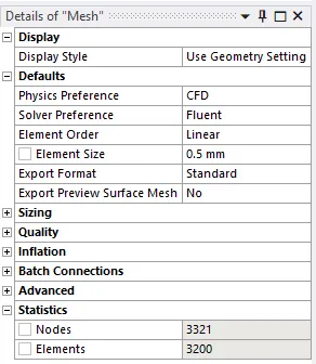
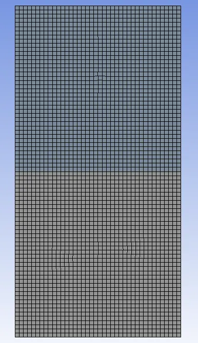
Mesh 0.5mm

Case 2

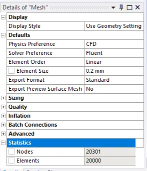
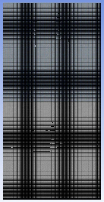
mesh0.2mm

Case 3

User defined fluid (density = 400 kg/m³, viscosity = 0.001 kg/m-s)

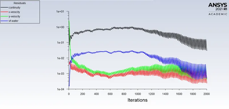
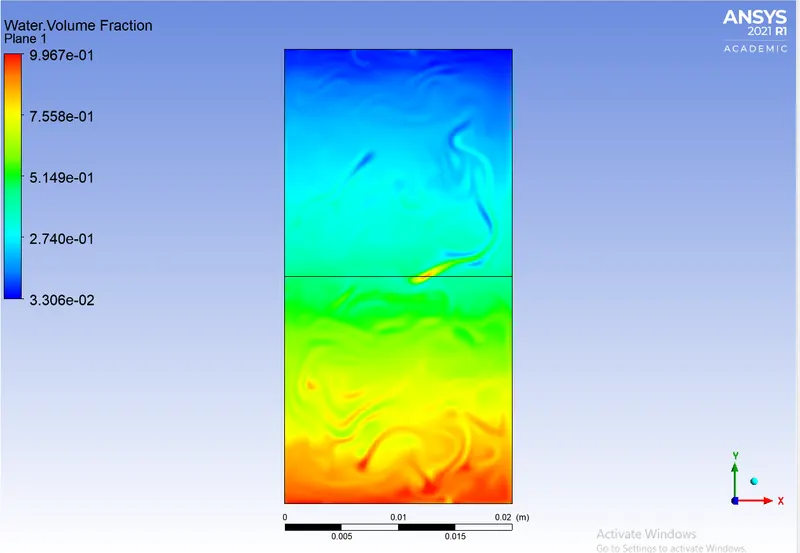
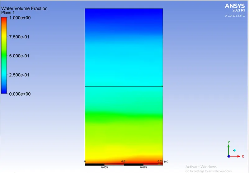
Results:

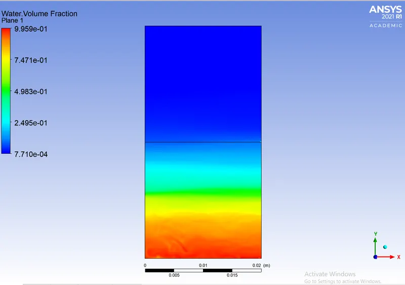
We can observe that as we increase our mesh quality, the mixing of both fluids gets smoother and realistic to the physical case.

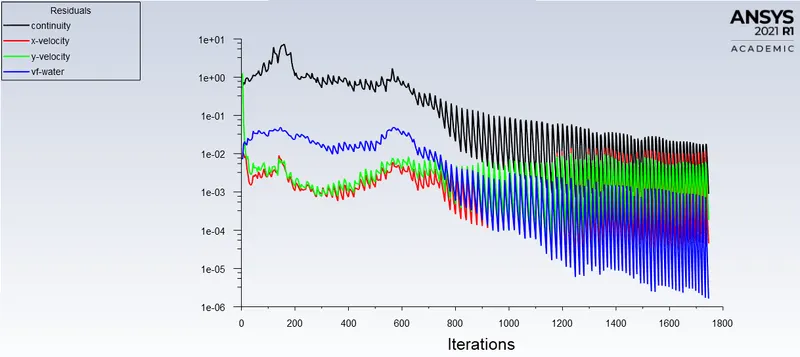
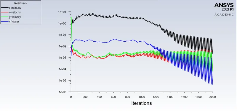
The reason why we won't use steady-state simulation in this condition because the difference between Steady-state and transient simulation is that in steady-state one can't see the small-time variation of instability.

Steady-state simulations are when we are more concerned about the final state results or equilibrium state, In this case, we are concerned to capture the transition of irregularities that starts developing when pouring high-density fluid upon the low-density fluid under the effect of gravity.

Hence transient analysis is a must in this case to capture the intermediate relations and behaviors of mixing fluid.

Atwood number

The Atwood number (A) is a dimensionless number in fluid dynamics used in the study of hydrodynamic instabilities in density stratified flows.

where

= density of heavier fluid

= density of lighter fluid

for case 1

Heavier fluid (water)

density 1 =998.2 kg/m^3

Lighter Fluid (Air)

density 2 =1.225 kg/m^3

Atw2ood number = 0.996

for case 3

Heavier fluid (water)

density 1 =998.2 kg/m^3

Lighter Fluid (User-defined fluid)

density 2 =400 kg/m^3

Atw2ood number = 0.427

When calculated Atwood number is close to 0, RT instability flows takes the form asymmetric finger of fluid, for Atwood number close to 1 the much lighter fluid below the heavier fluid takes the form of larger bubble-like plumes