Week 5 - Rayleigh Taylor Instability

Aim and Objective :

1. What are some practical CFD models that have been based on the mathematical analysis of Rayleigh Taylor waves? In your own words, explain how these mathematical models have been adapted for CFD calculations.
2. Perform the Rayleigh Taylor instability simulation for 2 different mesh sizes with the base mesh being 0.5 mm. Compare the results by showing the animations( Attach them from your google drive). Observe the differences in the animation and explain the effect of mesh size on simulation. Also, explain why a steady-state approach might not be suitable for these types of simulation.

[ Choose Air and Water for this simulation]

1. Run one more simulation with water and user-defined material(density = 400 kg/m³, viscosity = 0.001 kg/m-s) for refined mesh.
2. Define the Atwood Number. Find out the Atwood number for both the cases and explain how the variation in Atwood number in the above two cases affects the behaviour of the instability.

Introduction and Theory :

Rayleigh Taylor instability is phenomenon that occurs at the interference of fluid of different densities where the lighter fluid pushes the Havier fluid due to difference in density. it is the dynamic process where the system tries to reduce its potential energy initially the system is in state of hydrostatic equilibrium in which the heavy fluid sits top of lighter fluid in constant gravitational field. The ensuing turbulence and mixing as far-reaching consequences in many natural and man made flows, ranging from supernovae to inertial confinement fusion capsules.

Using this we are going to solve two different fluid behaviour with gravitation acting on it. For this simulation we goanna use multiphase , vof (volume of fraction) and many different techniques

Volume of fluid method :

The VOF method provides a simple and economical way to track free boundaries in two- or three-dimensional grids, and is more flexible and efficient than the finite-difference method in dealing with problems involving highly complex free surface configurations. It's a numerical method for tracking and locating a free surface. It belongs to the class of Eulerian methods which are characterized by a mesh that is either stationary or is moving in a certain prescribed manner to accommodate the evolving shape of the interface.

Practical CFD models based on mathematical analysis:

1. Kelvin Helmholtz instability: The Kelvin Helmholtz instability can occur when there is velocity shear in a single continuous fluid, or where there is a velocity difference across the interface between two fluids. An example is wind blowing over water: The instability manifests in waves on the water surface. More generally, clouds, the ocean, Saturn's bands, Jupiter's Red Spot, and the sun’s corona show this instability.

2. Richter-Meshkov instability: The Richter-Meshkov instability occurs when two fluids of different density are impulsively accelerated. Normally this is by the passage of a shock wave. The development of the instability begins with small amplitude perturbations which initially grow linearly with time. This is followed by a nonlinear regime with bubbles appearing in the case of a light fluid penetrating a heavy fluid, and with spikes appearing in the case of a heavy fluid penetrating a light fluid. A chaotic regime eventually is reached and the two fluids mix. This instability can be considered the impulsive-acceleration limit of the Rayleigh-Taylor instability. This instability is also seen in Magnetized Target Fusion. Mixing of the shell materialand fuel is not desired and efforts are made to minimize any tiny imperfections or irregularities which will be magnified by RMI.

3. Plateu-Rayleigh instability: the Plateu-rayleigh instability, often just called the Rayleigh instability explains why and how a falling stream of fluid breaks up into smaller packets with the same volume but less surface area. It is related to the Rayleigh-Taylor instability and is part of a greater branch of fluid dynamics concerned with fluid thread breakup. This fluid instability is exploited in the design of a particular type of ink jet technology whereby a jet of liquid is perturbed into a steady stream of droplets. The driving force of the Plateau–Rayleigh instability is that liquids, by virtue of their surface tensions, tend to minimize their surface area. A considerable amount of work has been done recently on the final pinching profile by attacking it with self-similar solutions.

Atwood number:

Atwood number is dimension less number in fluid dynamics used in study of hydrodynamic instability In density stratified flow it is dimensionless density ratio

Atwood number = (rho_1-rho_2)/(rho_1+rho_2)

Rho_1 is density of heavier fluid

Rho_2 is density of lighter fluid

Case 1 and case 2 where fluids are air and water atwood number is

Air density (lighter fluid): 1.225 kg/m3

Water density (heavier fluid) : 998.2 kg/m3

Atwood number = (998.2 – 1.225)/ (998.2+1.225)

= 0.9975

Case 3 where fluids are water and user defined atwood number is

Water density = 998.2

User defined material = 400

Atwood number = 598.2 /1398.2

= 0.4278

Solving and modelling approach :

Pre-processing:

To solve this simulation first we create the base line model in which first we creates the geometry in space claim using the two rectangles as two container containing two different fluid of different properties then we make them share there share topology so we can create the conformal mesh in between them.

Then moving forward we create the mesh in meshing module in which as our model is baseline model so we first create the model which consumes less computational power so we creates the mesh which is not too refined but should be good for simulation.so we create the mesh of element size 0.5 mm.

Now its time for setup so we do the actual setup which we requires in model further in which we set the boundary condition, model equation, method of solving, phases setting, patching, solvers etc lets discuss these things in setup part as now we focus on pre-processing. So we get the animation of baseline mesh in which we can see the result is not much defined and the interface thickness is on high.

So we again coming back to mesh we goes for another case where we reduce the element size of mesh to 0.3 and see the result where we can see the result is more defined and interference thickness is also reduced.

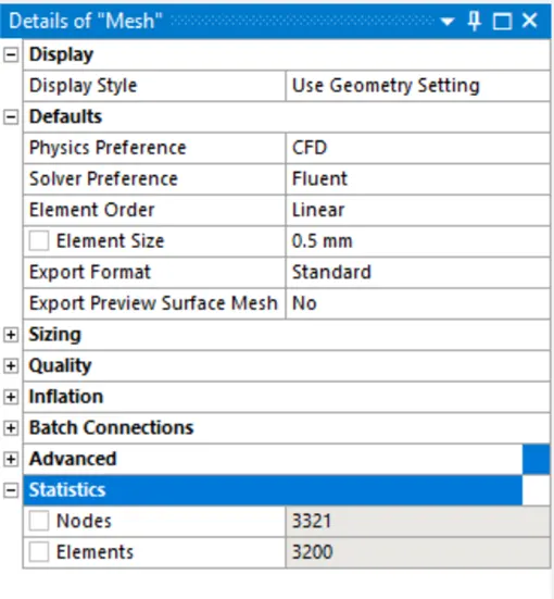
Fig 1. Mesh 0.5 case

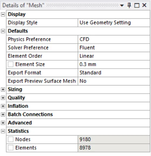
Fig 2. Mesh 0.3 case

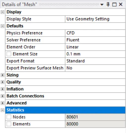
Fig 3. Mesh 0.1 case (most refined)

Setup :

In setup we first check in the gravity box as we have to deal with it in this case and our gravity is along the y axis so we provided there the gravity as -9.81

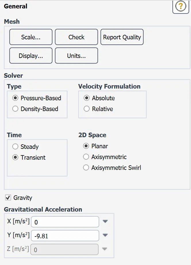
Fig 4. solver Setup

Moving forward as we have to focus on moment of fluids for each sec so we requires transient in time solver because steady deals with direct result where the result is prioritised. And pressure based solver as we no need of near the wall condition here.

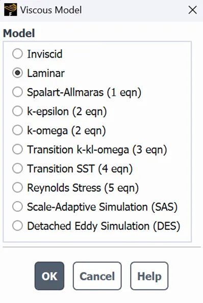
Fig 5. Viscous model setup

Then in viscous model we select the laminar model and we select multiphase here as we have to deal with the two different fluid in different phases. In that multiphase we select the two liquid we wanted in which phase (primary, secondary) here we have to choose those material which was in our material list in our case we choose water and air in first to case and water and user defined material in 3^rd case. Also in multiphase we have to select volume of fluid in model and implicit as volume fraction parameter and enter how many phase we have to deal with.

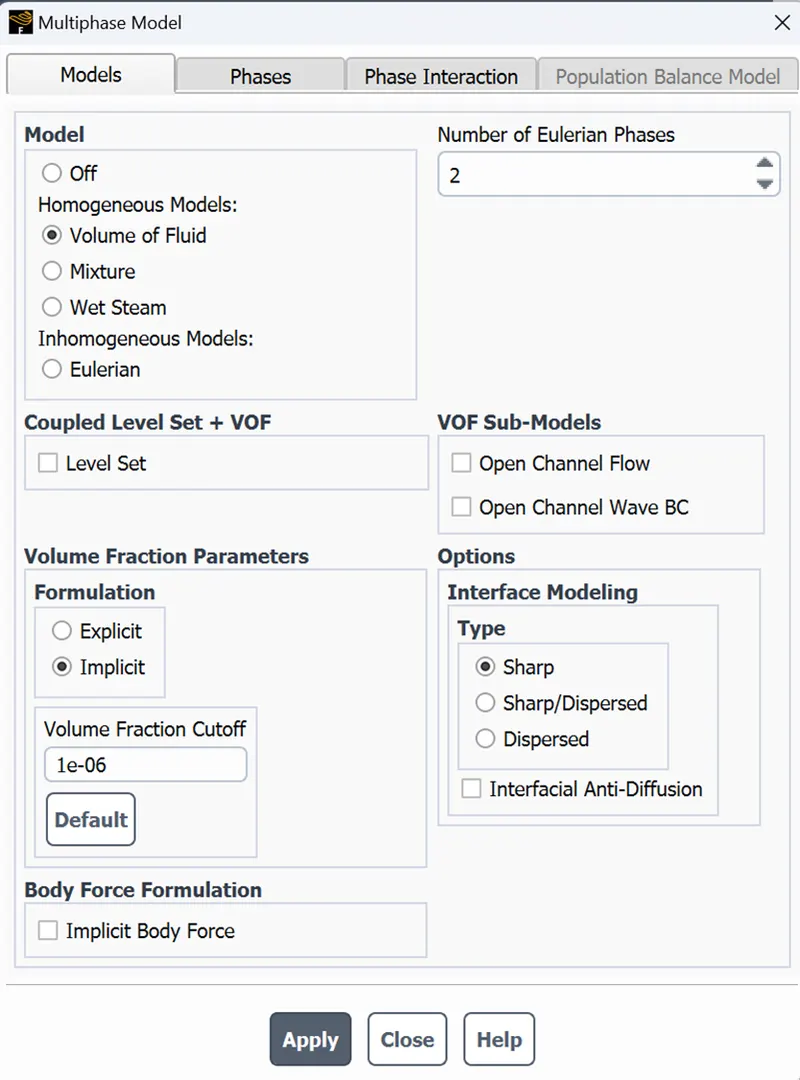
Fig 6. Multiphase model setup

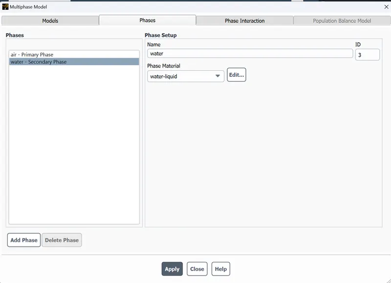
Fig 7. Phase selection for case 1 and 2

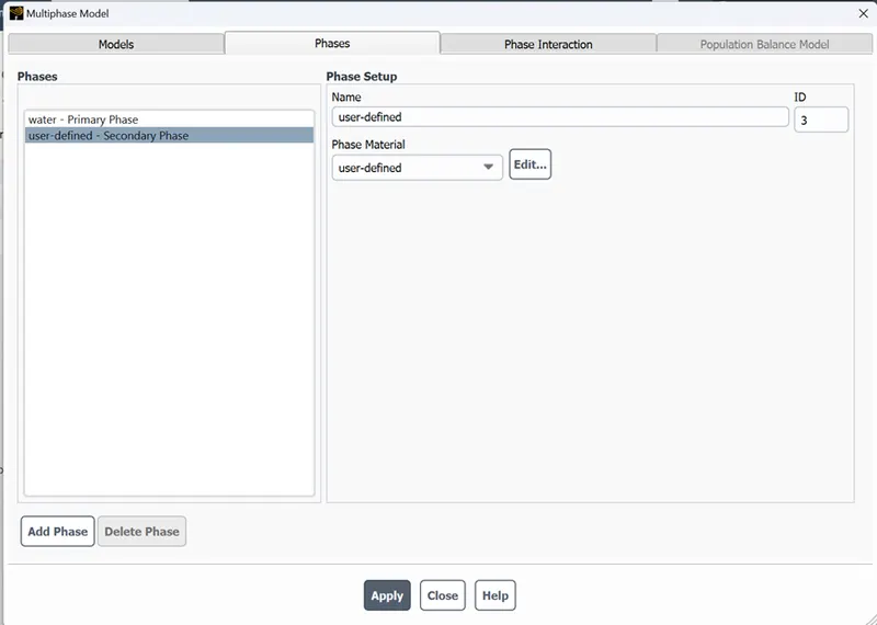
Fig 8. Phase selection for case 3

Now as we are not going to deal with the outcomes results and numbers hence we avoid the hybrid initialization and choose the standard initialization here.

After initializing we have to patch the fluid. Now what is patch so, patch is used to assign different values of particular variables into different cells in this challenge we use relative to cell option as we are dealing with moving reference frames. In this study we use patch because we need to assign different value of volume fraction to two different fluids. Here after initialization we define volume of fraction for water=1 and air = 0 and by this we end our setup of solver and run the calculation.

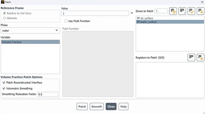
Fig 9. Patching of fluids

Results :

Result animation for case 1 mesh element size is 0.5 :

https://drive.google.com/file/d/1lZMyTuUG1H9R9ZPBgRtjJGA2I3GnatsH/view?usp=share_link

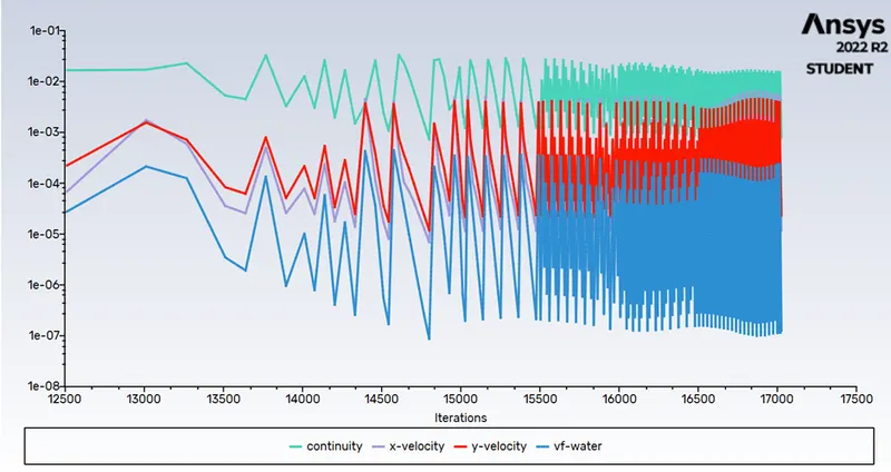
Fig 9. Scaled residuals for baseline mesh

Result animation for case 1 mesh element size is 0.3 :

https://drive.google.com/file/d/1Ne8-H40Bf-RJJcXXmsMwxoEx8Pf_UZUY/view?usp=share_link

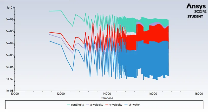
fig 10. Scaled residuals for mesh 0.3

Result animation for case 1 mesh element size is 0.1 here the material is change where density is 400 and viscousity is 0.001 :

https://drive.google.com/file/d/1IGEQOkmOOpqPAcea1VtGv4KTjownd_s_/view?usp=share_link

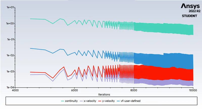
Fig 11. Scaled residuals for mesh 0.1

Conclusion :

In conclusion we can see as we reduce the mesh element size and increase the mesh refinement the results will be more defined and the interference thickness reduce with increase in mesh refinement