Week 5 - Rayleigh Taylor Instability

AIM :

To perform the Rayleigh Taylor instability simulation for two dimensional multiphase flow of two immiscible fluids (water and air in one case, water and user defined fluid for the other).

OBJECTIVES :

• To create two dimensional surfaces for the two fluid components in spaceclaim.
• To generate mesh with different mesh element size for different cases and perform the mesh independency study for those cases.
• To setup the simulation for capturing the Rayleigh Taylor instability between the two immiscible fluids which flows due to gravity.
• To create animation for visualising the Rayleigh instability on those fluids and to calculate the Atwood number for water and air, also water and user defined fluid.

INTRODUCTION :

In this project, we are going to perform the two dimensional simulation for two immiscible fluids that have different densities. Initially, the fluid with high density is placed at the top region while the fluid having lesser density at the bottom. Due to gravity, the heavy dense fluid flows downwards making the less dense fluid to go up. This causes the Rayleigh Taylor instability between the interface of those two fluids. This instability is captured from this simulation which set to run at transient state with maximum of 10 flow seconds in some cases which is more than enough for the two fluids to reach the steady state.

CFD MODELS BASED ON RAYLEIGH-TAYLOR WAVES :

Rayleigh-Taylor instability :

It is an instability of an interface between two fluids of different densities which occurs when the lighter fluid is pushing the heavier fluid. For example, If the water is suspended above oil which has less density than water, due to gravity, the heavier dense water flows downwards which makes the oil to go upwards. This behaviour is Rayleigh instability.

Richtmeyer-Meshkow instability :

This instability occurs when a shock wave interacts with an interface separating two different fluids or in other words when two fluids of different densities are impulsively accelerated.The development of instability begins with small amplitude which initially grow linear with time. This is followed by a nonlinear regime with bubbles appearing in the case of a light fluid penetrating a heavy fluid, and with spikes appearing in the case of a heavy fluid penetrating a light fluid. A chaotic regime eventually is reached and the two fluids mixThis instability can be considered the impulsive acceleration limit of the Rayleigh Taylor Instability.

Plateau-Rayleigh instability :

This instability explains why and how a falling stream of fluid breaks up into smaller packets with the same volume but different or small surface area.The driving force of this instability is that the liquids by virtue of their surface tensions ,tends to minimize their surface area .

Kelvin-Helmholtz instability :

This instability can occur when there is velocity shear in a single continuous fluid, or where there is a velocity difference across the interface between two fluids. For example, wind blowing over the water, cloud formation, etc.

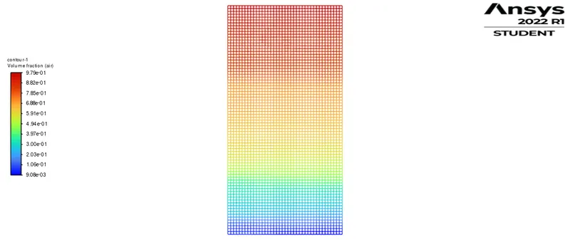
ATWOOD NUMBER :

It is a dimensionless number which is defined as the ratio of the difference between the heavier fluid density and the lighter fluid density to their sum. It used in the study of hydrodynamic instabilities in density stratified flows. It is an important parameter in the study of Rayleigh-Taylor instability and Richtmyer-Meshkov instability.

• Atwood number (A)=ρ1−ρ2ρ1+ρ2Atwood number (A)=ρ1-ρ2ρ1+ρ2

Where,

• ρ1=Density of the heavier fluidρ1=Density of the heavier fluid
• ρ2=Density of the lighter fluidρ2=Density of the lighter fluid

CALCULATION OF ATWOOD NUMBER :

1. For water and air,

Here, water is the heavier dense fluid compared to air, so, we take

Density of water,

ρ1=998.2 kg/m^3ρ1=998.2 kg/m^3

Density of air,

ρ2=1.225 kg/m^3ρ2=1.225 kg/m^3

We know that,

Atwood number (A)=ρ1−ρ2ρ1+ρ2Atwood number (A)=ρ1-ρ2ρ1+ρ2

A=998.2−1.225998.2+1.225A=998.2-1.225998.2+1.225

A=0.9975A=0.9975

2. For water and user defined fluid,

Density of user defined fluid,

ρ2=400 kg/m^3ρ2=400 kg/m^3

Density of water,

ρ1=998.2 kg/m^3ρ1=998.2 kg/m^3

Therefore,

A=998.2−400998.2+400A=998.2-400998.2+400

A=0.4278A=0.4278

• COURANT NUMBER (CFL NUMBER)-

In mathematics, the Courant-Friedrichs-Lewy condition is necessary to condition for convergence while solving certain partial differential equations numerically by the method of finite differences. It arises in the numerical analysis of explicit time-marching schemes when these are used for the numerical solution. As a consequence, the time step must be less than a certain time in many explicit time-marching computer simulations, otherwise, the simulation will produce an incorrect result. The condition is named after Richard Courant, Kurt Friedrichs, and Hans Lewy who described in 1928.

In 1D cells, to identify the courant number let's consider a rectangular cell. In that flow field, the fluid flows from left to right represented by U profile, and ΔxΔx represents the total length of the cell as shown in the figure. Over the time step delta T, the velocity approaches in the cell with the distance of Udeltat of the cell having the length of delta x across the cell. The bigger is the time step ΔtΔt further the distance covered by UΔtUΔt. Now the courant number defines as the ratio of the distance flow covered (UΔtUΔt) to the length of the cell (ΔxΔx) or The fraction of the cell that the flow moves across in the time step.

Co=FluidDistanceCellDistance=UΔtΔxCo=FluidDistanceCellDistance=UΔtΔx

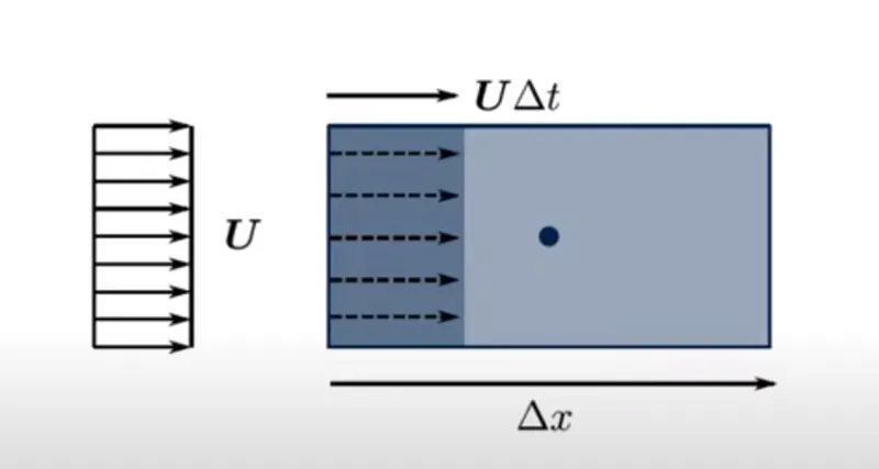
Fig No. 1. 1D cell representation in a rectangular format to compare the length scale.

If Co = 0.3 then the flow distance covers 30% of the length of the cell and if Co = 1.1 then the flow of fluid covers or surpasses the length of the cell in a single timestep.

In 3D, the system courant number behaves differently keeping the basic definition the same because of the irregular shape of the 3D cell or skewness in element quality. If the cells are not in perfect shape then the system of calculating courant number needs to modify accordingly for this purpose need to define the length of flow in a particular cell in the particular cell according to the orientation of the cell. The distance across the cell can be defined as -

Δx=CellVolumeTotalSurfaceArea=VAΔx=CellVolumeTotalSurfaceArea=VA

Total surface area can be defined as the sum of the surface area/ length of the face of the cell.

A = A1 + A2 + A3 + ........... + An.

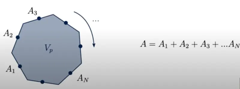
Fig No.2. 3D cells surface area calculation and the orientation calculation complexity.

Now for the velocity, have to find the velocity normal to the face. Also need to understand the condition of conservation of mass. This creates a problem of the sum of velocity normal results in zero. To avoid this needs to take magnitude and divide with 1/2 to get the actual velocity flux normal to face. The final definition of courant number for an arbitrary shaped 3D cell can be represented as,

Velocity flux = ∑(12⋅Uf⋅nf)∑(12⋅Uf⋅nf)

Co=12⋅Δt⋅(∑∣Uf⋅nfVp)Co=12⋅Δt⋅(∑∣Uf⋅nfVp)

The courant number should be considered as a field because every cell in the mesh has a different courant number. Hence, it is a field and can be plotted like any other variable such as temperature, velocity, and pressure. Most often the maximum courant number should be below 1.0.

• TIMESTEPPING SCHEME -

Fixed time-stepping - Choose a time step size ΔtΔt then CFD solver computes the flow field U and compute Co courant number for every cell. Then proceed to the next iteration keeping ΔtΔt the same also ΔxΔx will remain fixed over a simulation. The CFD solver continues the procedure, if the courant number is too large the solution may diverge or Crashdown. Now have to go back to change manually the timestep and rerun the simulation.

Adjustable time-stepping - In such scenarios, to avoid the complexity of time stepping better option is to use an automatic adjustable time-stepping scheme rather than a fixed time step. In the adjustable time-stepping scheme, initial time step size ΔtΔt and maximum courant number Comax are provided. CFD solver computes flow field U then finds Co. If Co > Comax then reduces the time step ΔtΔt for the next iteration. The reduction in time step ΔtΔt carried out by the simple way,

Δtn=Δtold⋅ComaxCoΔtn=Δtold⋅ComaxCo

But it creates the problem of very rapidly changing the time step which creates oscillation and it may diverge the solution or disturb the accuracy. Now in such case have to use either relaxation or limiting to prevent large change in ΔtΔt.

• GEOMETRY DETAILS -

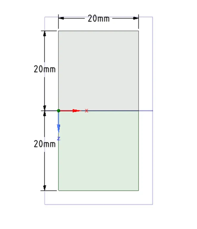
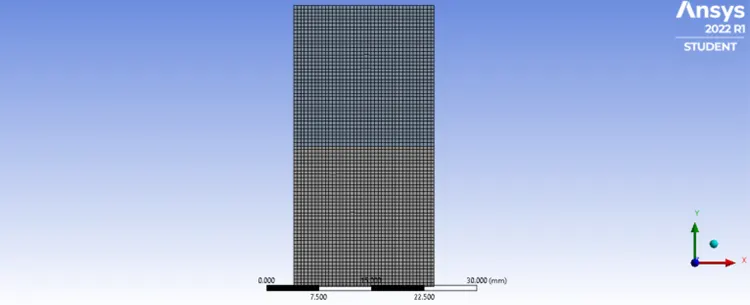
1. BASELINE MESH AND ITS MESH METRICS AT 0.5MM BASE MESH -
2. 

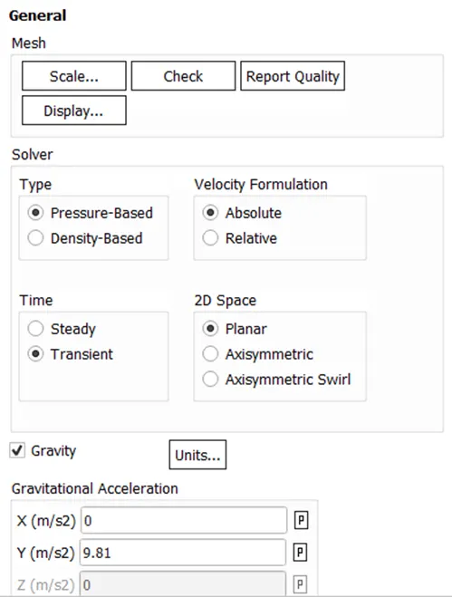
• SETUP -

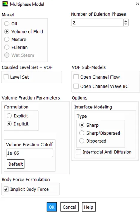
Multiphase model.

In the multiphase model, the implicit method for the formulation is used by keeping on the body force formulation.

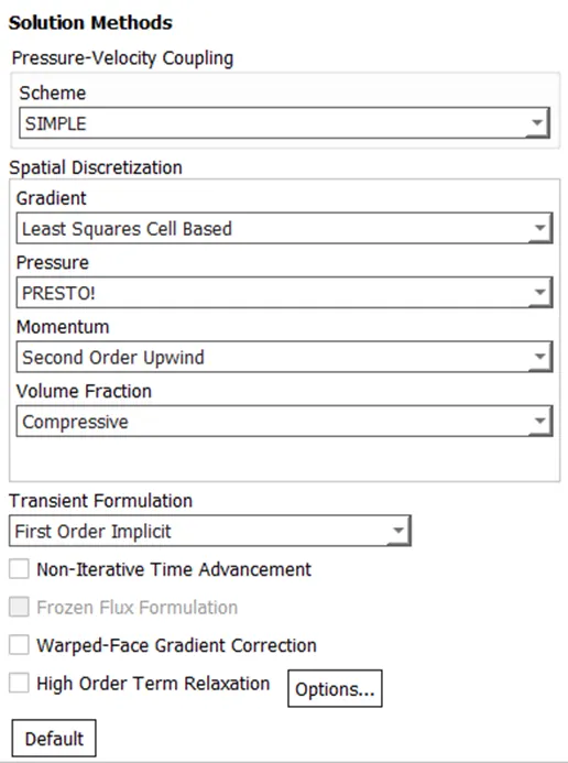
• RESULTS -

1. The RTI analysis under the gravitational acceleration of the 9.81m/s^2 at 0.5 mm base mesh by providing default material of air and water.

• CONCLUSION -

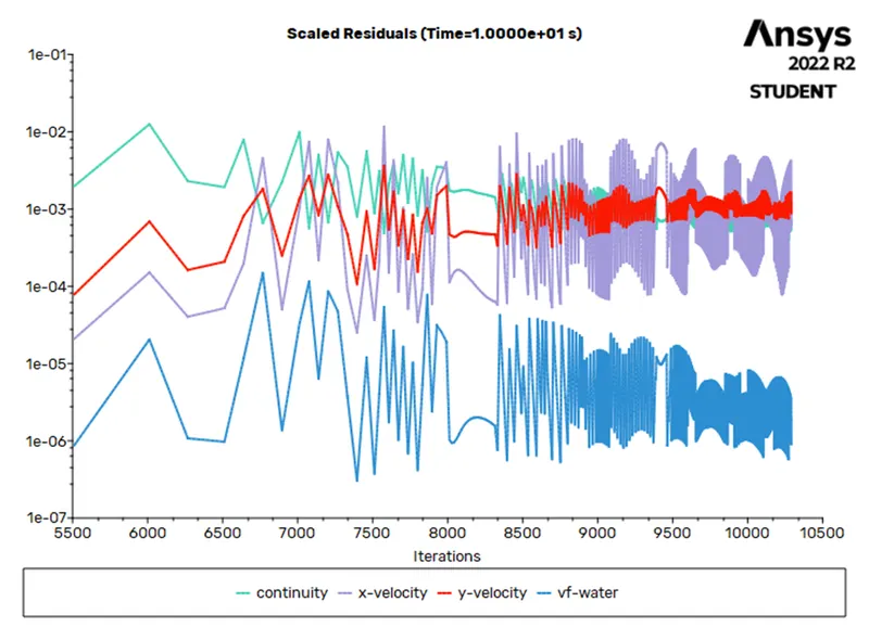
1. Choosing the wrong timestep leads to floating-point error.
2. The way to smaller timesteps will not provide the solution at all. To avoid such a problem adjustable time step should use.
3. Instabilities are captured when the mesh size is smaller but, it certainly needs more time for calculations.
4. The third case shows larger turbulence generated and vortices form.
5. In all simulation results, when the fluid gets to settle down one can observe that the mixing and diffusion of the fluid at the center of the geometry.
6. It is quite difficult to understand in the first two cases when the air and water are used as the fluid when the solution gets to settle down one can observe the mixing of phases in the center or the reduction in the number of fluidswhich cannot happen at normal circumstances.