Week 5 - Rayleigh Taylor Instability

Rayleigh Taylor Instability

Objectives:

1. To explore practical CFD models that have been based on the mathematical analysis of Rayleigh Taylor waves.

2. Perform the Rayleigh Taylor instability simulation for 2 different mesh sizes with the base mesh being 0.5 mm. Compare the results by showing the animations. Observe the differences in the animation and explain the effect of mesh size on simulation. Also, explain why a steady-state approach might not be suitable for these types of simulation.

3. Setup a simulation with water and user defined material (density = 400 kg/m³, viscosity = 0.001 kg/m-s) for refined mesh.

4. Find out the Atwood number for both the cases and explore the variation in Atwood number in the above two cases and its effects in the behavior of the instability.

Rayleigh Taylor Waves:

The Rayleigh–Taylor instability, is an instability of an interface between two fluids of different densities which occurs when the lighter fluid is pushing the heavier fluid. There are few other instabilities based out of Rayleigh Taylor and found practical application in certain areas;

• Kelvin–Helmholtz instability - typically occurs when there is friction velocity in a single continuous fluid, or additionally where there is a velocity difference across the interface between two fluids. A common example is seen when wind blows across a water surface in which the instability constant manifests as waves.
• Saffman-Taylor instability - also known as viscous fingering, is the formation of patterns in a morphologically unstable interface betweeen two fluids in a porous medium. This situation is most often encountered during drainage processes through media such as soils.
• Richtmyer–Meshkov instability (RMI) occurs when two fluids of different density are impulsively accelerated. Normally this is by the passage of a shock wave. The development of the instability begins with small amplitude perturbations which initially grow linearly with time. This is followed by a nonlinear regime with bubbles appearing in the case of a light fluid penetrating a heavy fluid, and with spikes appearing in the case of a heavy fluid penetrating a light fluid. A chaotic regime eventually is reached and the two fluids mix. This instability can be considered the impulsive-acceleration limit of the Rayleigh–Taylor instability.
• Plateau Rayleigh instability - explains why and how a falling stream of fluid breaks up into smaller packets with the same volume but less surface area.This fluid instability is exploited in the design of a particular type of ink jet printing technology.

Atwood Number:

As the RT instability develops, the initial perturbations progress from a linear growth phase into a non-linear growth phase, eventually developing "plumes" flowing upwards (in the gravitational buoyancy sense) and "spikes" falling downwards. In the linear phase, the fluid movement can be closely approximated by linear equations, and the amplitude of perturbations is growing exponentially with time. In the non-linear phase, perturbation amplitude is too large for a linear approximation, and non-linear equations are required to describe fluid motions. In general, the density disparity between the fluids determines the structure of the subsequent non-linear RT instability flows (assuming other variables such as surface tension and viscosity are negligible here). The difference in the fluid densities divided by their sum is defined as the Atwood Number, A. For A close to 0, RT instability flows take the form of symmetric "fingers" of fluid; for A close to 1, the much lighter fluid "below" the heavier fluid takes the form of larger bubble-like plumes.

A= `(rho (water)-rho(air))/(rho (water)+rho(air))`

Geometry:

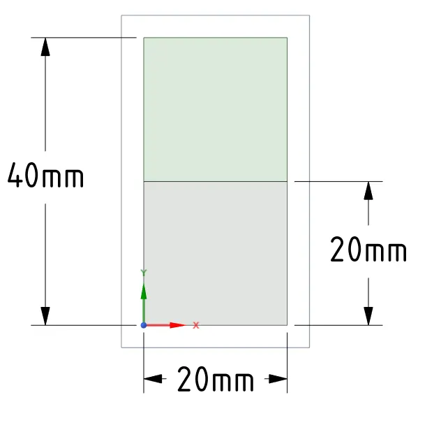
The top part of the geometry is occupied by water and the bottom part of the geometry is occupied by air.

Meshing:

Baseline Case: (Element size 0.5 mm)

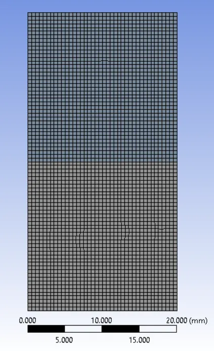
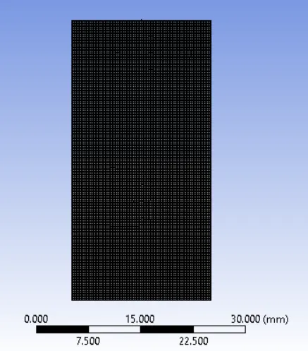
Refined Case : (Element size 0.2 mm)

Case setup:

• Transient
• Solver: Pressure based (since the flow is of low speed)
• Gravity: 9.81 m/s2 (along -Y axis)
• Viscous model: Laminar
• Multiphase: on (Air and Water)

Fluid Properties:

Air: Density- 1.225 kg/m3, Viscosity - 1.7894e-05 (kg/m-s)

Water: Density- 998.2 kg/m3, Viscosity - 0.001003 (kg/m-s)

Output Plots:

Case 1:

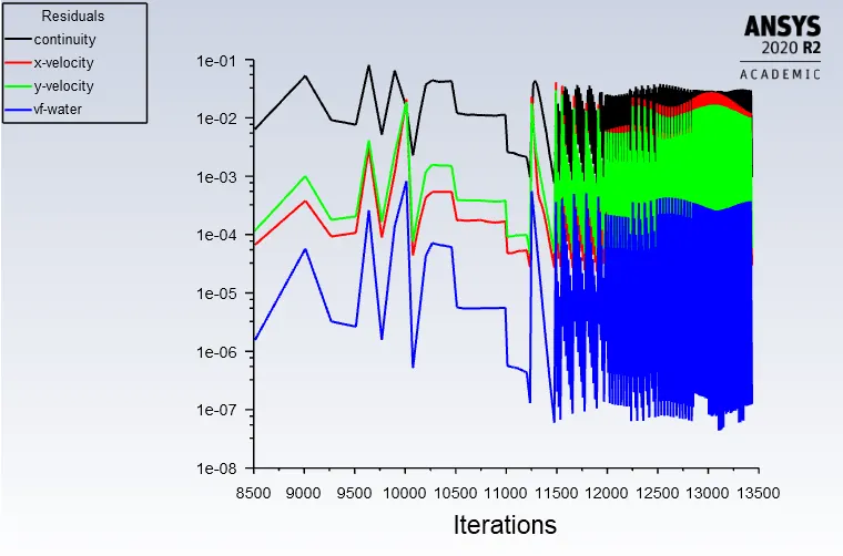
Residual Plot for Baseline mesh setup:

(Time step: 1500, Time step size: 0.005, Iterations/Time step: 20)

Contour Plot of Rayleigh instability :

Click Here for Rayleigh Instability of Baseline setup (0.5mm) with default fluid

Case 2:

Residual Plots for Refined mesh setup: (Time step: 750, Time step size: 0.005, Iterations/Time step: 20)

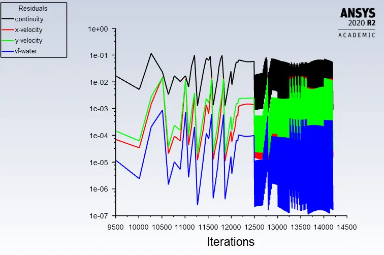
Contour Plot of Rayleigh instability :

Atwood Number A = (rho (water)-rho (air))/(rho (water)+rho (air)) = (998.2-1.225)/(998.2+1.225) =0.99

Click Here for Rayleigh Instability with 0.2mm mesh (Default air and water)

Case 3:

Residual Plot for Refined mesh setup with custom fluid:

(Time step: 750, Time step size: 0.005, Iterations/Time step: 20)

Here,

Custom fluid: Density = 400 kg/m³, viscosity = 0.001 kg/m-s

Water: Density= 998.2 kg/m3, Viscosity = 0.001003 (kg/m-s)

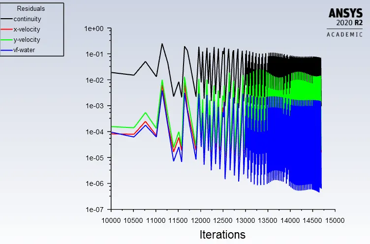
Contour Plot of Rayleigh instability:

Atwood Number A = (rho (water)-rho (air))/(rho (water)+rho (air)) = (998.2-400)/(998.2+400) =0.42

Click Here for Rayleigh Instability with 0.2 mm mesh (Custom fluid)

Inference:

• In the refined cases 2 and 3, Atwood numbers are 0.99 and 0.42 respectively. As per [1], For A close to 0, RT instability flows take the form of symmetric "fingers" of fluid; for A close to 1, the much lighter fluid "below" the heavier fluid takes the form of larger bubble-like plumes. It is evident from the below contour snaps from case 2 and 3.

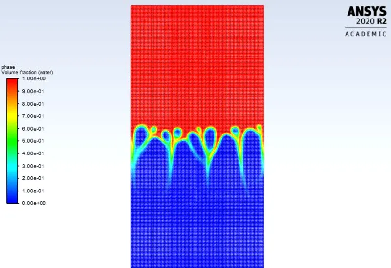
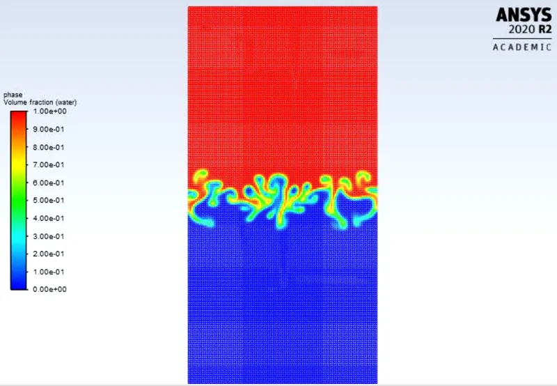
Fig. A=0.99(Left) Plumes, A=0.42 (Right) Fingers

• Steady state simulation for capturing Rayleigh instability is not suitable as the variations are not linear completely. The initial perturbations progress from a linear growth phase into a non-linear growth phase.

References:

[1] https://en.wikipedia.org/wiki/Rayleigh%E2%80%93Taylor_instability