Multiphase flow simulation on Rayleigh-Taylor Instability
Objective:
- What are some practical CFD models that have been based on the mathematical analysis of Rayleigh Taylor waves? In your own words, explain how these mathematical models have been adapted for CFD calculations.
- Perform the Rayleigh Taylor instability simulation for 2 different mesh sizes with the base mesh being 0.5 mm. Compare the results by showing the animations( Attach them from your google drive). Observe the differences in the animation and explain the effect of mesh size on simulation. Also, explain why a steady-state approach might not be suitable for these types of simulation.[ Choose Air and Water for this simulation]
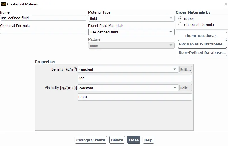
- Run one more simulation with water and user-defined material(density = 400 kg/m3, viscosity = 0.001 kg/m-s) for refined mesh.
- Define the Atwood Number. Find out the Atwood number for both the cases and explain how the variation in Atwood number in the above two cases affects the behavior of the instability.
Solutions:
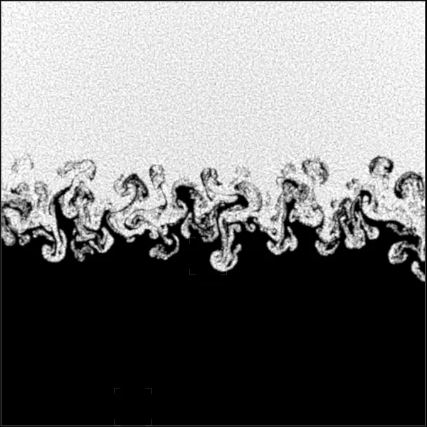
Here we are going to perform a very interesting flow pattern simulation where more than one phase of fluid is involved. Usually, we call it a multi-phase simulation to understand fluid behavior and its properties. One such behavior is having instability between the fluid at the interfacial boundary layer between 2 phases under the influence of a gravitational field. And we call it as Rayleigh-Taylor instability.
Before we hop on to explain the instability, we are going to understand what rayleigh-Taylor instability is and what are models are there to perform for multiphase simulations.
Rayleigh-Taylor instability.
The Rayleigh-Taylor instability (RTI) is a fundamental fluid dynamical phenomenon that occurs at the interface between a dense fluid supported by a lighter fluid under gravity, or, equivalently, in a system that is accelerating in the direction of the denser fluid. An example is the instability of a layer of brine above a layer of freshwater. The RTI has remained topical since the initial work of Lord Rayleigh and the investigations of Taylor and Lewis. Reasons for this include its common occurrence in industrial applications involving, for example, thin-film flows, pool boiling, and aerosol transport, as well as its intrinsic mathematical value.
It manifests in several natural physical phenomena including, for example, the finger-like structures of the Crab nebula, created by the acceleration of pulsar winds through a dense supernova remnant and salt tectonics, where deep salt sediments protrude upwards through the denser rock into finger-like “diapirs”. The RTI also constrains efforts to generate power from inertial confinement fusion, where, during the implosion of the target, instabilities develop at the interface between the vaporized shell and the fuel core, limiting the efficiency of the reaction. These examples illustrate the importance of furthering our understanding and our ability to influence the RTI through means beyond, for example, imposing an initial density difference. In particular, there are many situations in which it is desirable to stabilize the system against RTI, as in inertial confinement fusion.
The Euler-Euler approach
In the Euler-Euler approach, the different phases are treated mathematically as interpenetrating continua. Since the volume of a phase cannot be occupied by the other phases, the concept of phasic volume fraction is introduced. These volume fractions are assumed to be continuous functions of space and time and their sum is equal to one. Conservation equations for each phase are derived to obtain a set of equations, which have a similar structure for all phases. These equations are closed by providing constitutive relations that are obtained from empirical information, or, in the case of granular flows, by application of kinetic theory.
In ANSYS FLUENT, three different Euler-Euler multiphase models are available: the volume of fluid (VOF) model, the mixture model, and the Eulerian model.
The VOF Model
The VOF model is a surface-tracking technique applied to a fixed Eulerian mesh. It is designed for two or more immiscible fluids where the position of the interface between the fluids is of interest. In the VOF model, a single set of momentum equations is shared by the fluids, and the volume fraction of each of the fluids in each computational cell is tracked throughout the domain. Applications of the VOF model include stratified flows, free-surface flows, filling, sloshing, the motion of large bubbles in a liquid, the motion of liquid after a dam break, the prediction of jet breakup (surface tension), and the steady or transient tracking of any liquid-gas interface.
The Mixture Model
The mixture model is designed for two or more phases (fluid or particulate). As in the Eulerian model, the phases are treated as interpenetrating continua. The mixture model solves for the mixture momentum equation and prescribes relative velocities to describe the dispersed phases. Applications of the mixture model include particle-laden flows with low loading, bubbly flows, sedimentation, and cyclone separators. The mixture model can also be used without relative velocities for the dispersed phases to model homogeneous multiphase flow.
The Eulerian Model
The Eulerian model is the most complex of the multiphase models in ANSYS FLUENT. It solves a set of momentum and continuity equations for each phase. Coupling is achieved through the pressure and interphase exchange coefficients. The manner in which this coupling is handled depends upon the type of phases involved; granular (fluid-solid) flows are handled differently than nongranular (fluid-fluid) flows. For granular flows, the properties are obtained from the application of kinetic theory. Momentum exchange between the phases is also dependent upon the type of mixture being modeled. ANSYS FLUENT's user-defined functions allow you to customize the calculation of the momentum exchange. Applications of the Eulerian multiphase model include bubble columns, risers, particle suspension, and fluidized beds.
2. Perform the Rayleigh Taylor instability simulation for 2 different mesh sizes with the base mesh being 0.5 mm. Compare the results by showing the animations( Attach them from your google drive). Observe the differences in the animation and explain the effect of mesh size on simulation. Also, explain why a steady-state approach might not be suitable for these types of simulation. Choose Air and Water for this simulation
We are going to perform a Rayleigh-Taylor instability simulation in ANSYS-FLUENT with 2 different cases with different mesh sizes.
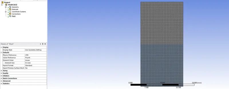
CASE 1: Baseline mesh is 0.5mm with 20x20mm two-phase squares
First, we build geometry
We run space claim to create the geometry and this is what this looks like below and then we take it to fluent. In space claim, we used different tools to create 2 phases. First, we use the SKETCH tool to create 2 boxes one on another and then we PULL to create the surface out of it.


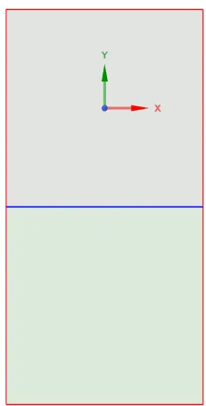
By enabling the sharing topology we are able to exchange information and we are able to see the mixing of two phases. And we know mesh the geometry with 0.5mm element size.
Now we gonna get ahead with FLUENT and set up and run the simulations.
we are going for transient state simulation and not a steady-state simulation as we need to observe the flow phenomenon with each and every time step and we are not interested in the end result of the instability. We are more into " How we get instability with respect to time " than "what do we get at the instability". The result is always visual and in a steady state, we are not able to observe the changes made at every time step. that is why we are going for transient state simulations.
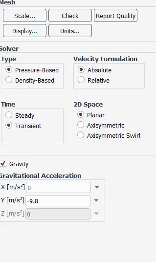
And we take gravity -9.8 as gravitational field acting at the -ve axis of Y, followed by and simple lamina viscous model with a multiphase model of VOF. The method we use here is the volume of fluid.
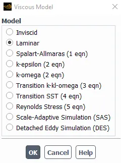
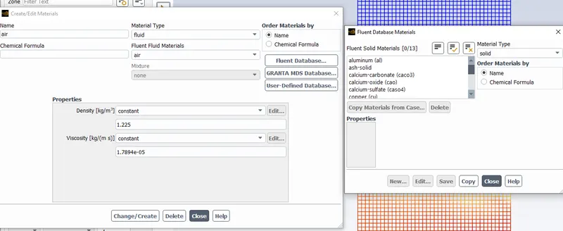
And we then deleted th materials to be going for.
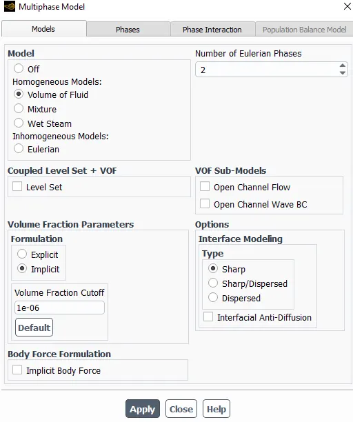
NOTE: THIS RECENT VERSION OF ANSYS FLUENT
So here they have changed the PHASES section and added it to the MULTIPHASE FLOW tool itself If you are able to go on the right side of the subsection.
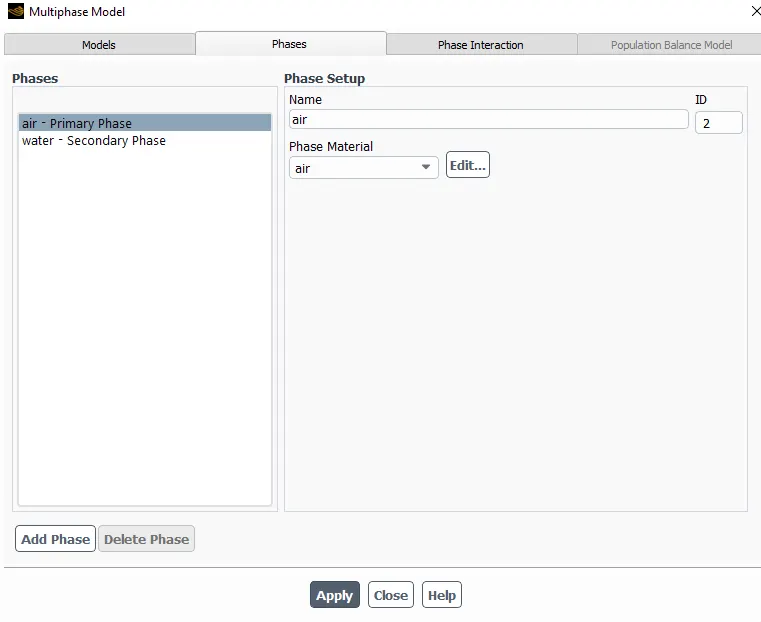
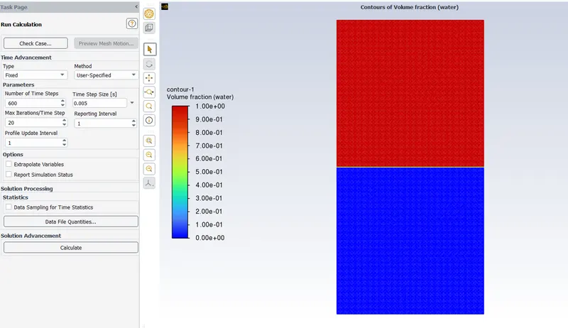
Here you can add which phase is which phase to the solver to understand for simulations. And we INITIALIZE the setup for simulation in time steps so every time step size is 0.005s. And we PATCH it with water and user-defined fluid.
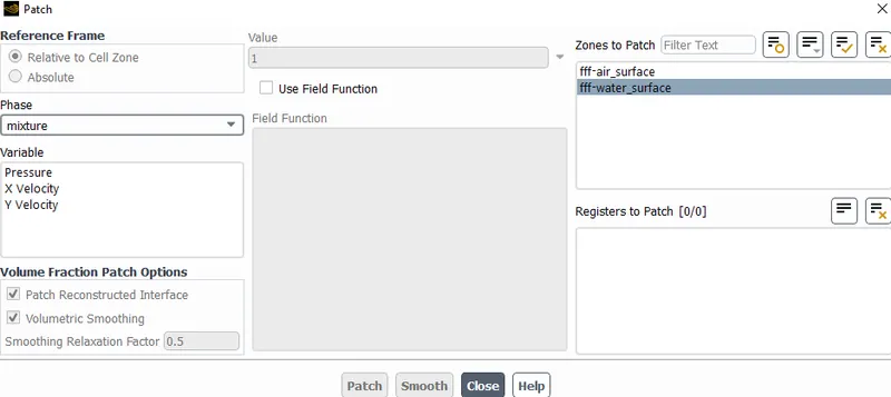
and we run the simulations for 500 iterations first. Observe the pattern with the time steps.
again NOTE:
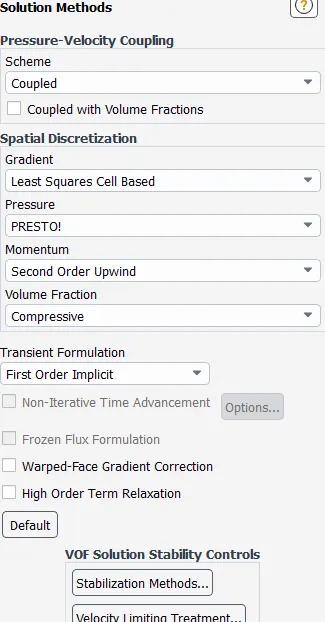
WE ENCOUNTERED THE FLOATING-POINT EXCEPTION ERROR, It seems we are observing divergence as the solver detects arithmetic operations. In that case, there are a lot of steps to safely troubleshoot this and solve it. But here in our case we actually preferred changing the from a SIMPLE method to COUPLED method scheme which helped out the issue to resolve. Here we have upwind scheme solutions.
OUTPUT:
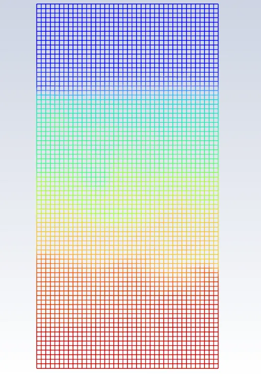
CASE 2: Steps are performed exactly as BASELINE MESH 0.5mm but we made changes in MESH as 0.01mm in this case.
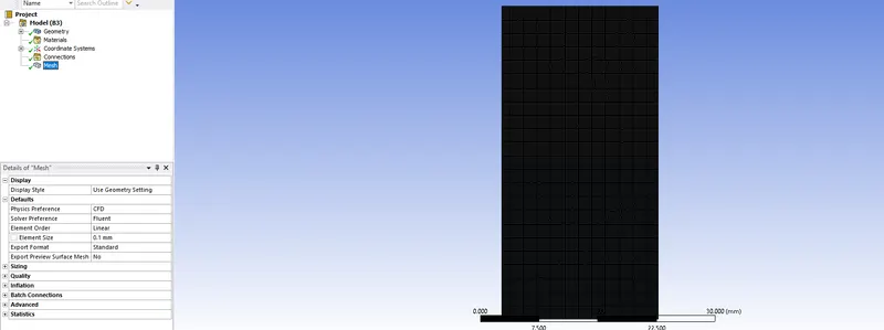
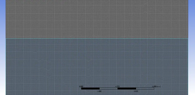
And then we take this to fluent where we run the simulation for 500 iterations and observe the pattern.
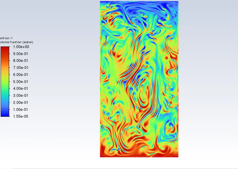
3. Run one more simulation with water and user-defined material(density = 400 kg/m3, viscosity = 0.001 kg/m-s) for refined mesh.
4. Define the Atwood Number. Find out the Atwood number for both the cases and explain how the variation in Atwood number in the above two cases affects the behavior of the instability
The Atwood number is a dimensionless number in fluid dynamics used in the study of hydrodynamic instabilities in density stratified flows. It is a dimensionless density ratio related to the density of the heavier fluid and the density of the lighter fluid. (The difference in the fluid densities divided by their sum). Atwood number is an important parameter in the study of Rayleigh–Taylor instability. For Atwood number close to 0, RT instability flows take the form of symmetric “fingers” of fluid; for Atwood number close to 1, the much lighter fluid “below” the heavier fluid takes the form of larger bubble-like plumes.
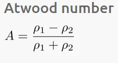
| A | Atwood number (dimensionless) |
| ρ1 | The density of the heavier fluid (kg/m3) |
| ρ2 | The density of the lighter fluid. (kg/m3) |
CASE 1: 0.5mm mesh
ρ1 = Water 997kg/m^3 ρ2 =Air 1.255Kg/m^3
A = 0.95
CASE 2: 0.1mm refined with User-defined fluid.
ρ1 = Water 997kg/m^3 ρ2 =UDF 400Kg/m^3
A = 0.42
Conclusion: For Atwood number close to 0, RT instability flows take the form of symmetric “fingers” of fluid; for Atwood number close to 1, the much lighter fluid “below” the heavier fluid takes the form of larger bubble-like plumes. Here in our 2 cases, the water and air case Atwood number is closer to 1 that's why we are able to see huge bubble formation at the starting time steps.
References: