Prandtl Meyer Shock problem
Objective:
1. Shock flow boundary conditions
Do a literature search on what BC's are typically used for shock flow problems
2. What is a shock wave?
In your own words, describe the physics behind shock waves
3. Effect of SGS parameter on shock location (Sub-Grid Scaling).
In the Prandtl Meyer shock problem, look at the effect of SGS temperature value on cell count and the shock location
It is expected to show the mesh generation using ParaView.
Also, create animation and upload it on Youtube and provide the Youtube link for animation in your report.
Solution:
Here we are going to perform the Prandtl Meyer shock problem. Before jumping into the analysis part, we need to undertsnad what shock wave is and what Boundary conditions are required to understand flows in Subsonic medium.
1. Shock flow boundary conditions
A literature search on what BC's are typically used for shock flow problems?
Boundary conditions (b.c.) are constraints necessary for the solution of a boundary value problem. A boundary value problem is a differential equation (or system of differential equations) to be solved in a domain on whose boundary a set of conditions is known.
Types of boundary condition.
Both ordinary and partial differential equations need boundary conditions to be solved. Different types of boundary conditions can be imposed on the boundary of the domain (Figure 1). The choice of the boundary condition is fundamental for the resolution of the computational problem: a bad imposition of b.c. may lead to the divergence of the solution or to the convergence to a wrong solution.
1. Dirchlet boundary condition
2. Neumann Boundary condition
3. Robin Boundary condition
4. Mixed boundary condition
5. Cauchy boundary condition
But the boundaries that are required for subsonic flow are as follows:
Dirichlet boundary conditions
In computational fluid mechanics, the classical Dirichlet boundary condition consists of the value of velocity and/or pressure to be taken by a certain set of nodes. It is common to refer to some sets of b.c. according to the following terminology:
- slip boundary condition: the velocity normal to the boundary is set to zero, while the velocity parallel to the boundary is let free
- no-slip boundary condition: both the velocity normal to the boundary and the velocity parallel to the boundary are set equal to zero.
At least one homogeneous b.c. on the pressure (i.e. p=0) has to be imposed as a reference for open domains, for instance, in the highest boundary of the air domain.
Neumann boundary conditions
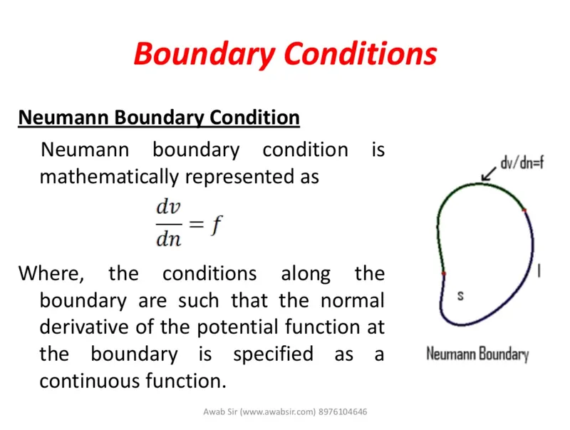
In mathematics, the Neumann (or second-type) boundary condition is a type of boundary condition, named after carl Neumann When imposed on an ordinary or a partial differential condition, the condition specifies the values in which the derivative of a solution is applied within the boundary of the domain. It is possible to describe the problem using other boundary conditions: a Dirichlet boundary condition specifies the values of the solution itself (as opposed to its derivative) on the boundary, whereas the Cauchy, mixed, robin boundary condition are all different types of combinations of the Neumann and Dirichlet boundary conditions.
Constraints on the derivative of velocity or pressure fields are mainly used in two cases. The first case is the application of a symmetry plane, thus:
Since this condition is always applied in addition to a Dirichlet b.c. it is naturally satisfied. The second application is the modeling of wall friction, in the case when it is proportional to the strain rate:
Mixed Boundary Condition
It consists of applying different types of boundary conditions in different parts of the domain. It is important to notice that boundary conditions must be applied on the whole boundary: the “free” boundary is anyways subjected to a homogeneous Neumann condition. The mixed boundary condition differs from the Robin condition because the latter consists of different types of boundary conditions applied to the same region of the boundary, while the mixed condition implies different types of b.c. applied to different parts of the boundary.
2. What is a shock wave?
In your own words, describe the physics behind shock waves
Shock waves are steep wavefronts that propagate in compressible fluids in which convection dominates diffusion. They are fundamental in nature, especially in high-speed fluid flows. Examples include transonic and/or supersonic shocks formed by supersonic flows impinging onto solid wedges, transonic shocks around supersonic or near-sonic flying bodies, bow shocks created by solar winds in space, blast waves caused by explosions and other shocks due to various natural processes. When a shock hits an obstacle, or a flying body meets a shock, shock reflection/diffraction phenomena occur.
Shock waves are steep wavefronts that are fundamental in nature, especially in high-speed fluid flows. When a shock hits an obstacle, or a flying body meets a shock, shock reflection/diffraction phenomena occur. In particular, these shock problems include von Neumann's problem for shock reflection–diffraction by two-dimensional wedges with concave corner, Lighthill's problem for shock diffraction by two-dimensional wedges with convex corner, and Prandtl-Meyer's problem for supersonic flow impinging onto solid wedges, which are also fundamental in the mathematical theory of multidimensional conservation laws.
Prandtl-Meyer Expansion Fan
In this section we analyze supersonic flows with larger deflections, dealing first with expansion turns in which the change in inclination of the flow is away from the flow and is thus an expansion deflection. In the previous section the flow deflection was denoted by θ and defined as positive into the flow; however, in the present context of an expansion deflection, it will avoid confusion if we define a new variable, θ∗ = −θ so that θ∗ is positive in this context. Then, examining the flow as sketched in Figure 1 it is clear that a gradual deflection will generate a set of Mach waves which diverge with distance from the surface. This is called an expansion fan, a rarefaction fan or a Prandtl-Meyer fan. Since it is comprised of Mach waves such
a flow will be isentropic. Moreover, if we pan out from the perspective of Figure 1 as depicted in Figure 2 the expansion fan will be seen to emanate from the vertex and the flow will be isentropic. Consequently
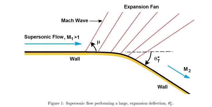
Figure 1: Supersonic flow performing a large, expansion deflection, θ∗
T
the relation between the small changes in the inclination, dθ∗, and the change in the Mach number, dM,
will be given by equation (Bok9) or
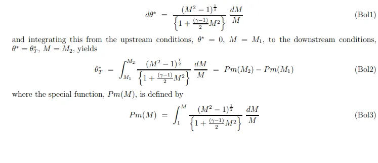
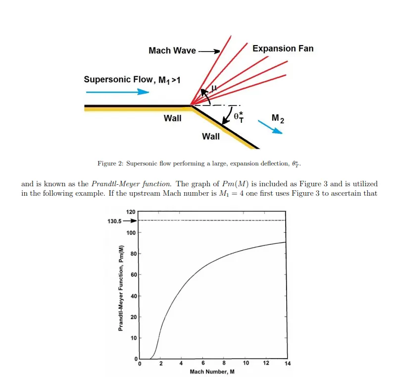
Pm(M1) = 65o. Then, if the deflection angle θ∗
T = 30o, it follows from equation (Bol2) that Pm(M2) = 95o and, using Figure 3 for a second time, that M2 ≈ 8. Moreover, since the process is isentropic, the tables and figures included in section (Boe) (Figures 1, 2 and 3 of section (Boe)) can then be used to find the relations between the pressures, temperatures and densities upstream (M = M1) and downstream (M = M2) of the expansion fan. Note from Figure 3 that the Prandtl-Meyer Function, Pm(M), has a maximum value of about 130.5 degrees. This implies that, for a given upstream Mach Number, M1, there is a maximum angle that the flow can negotiate. For example, for M1 = 4 and Pm(M1) = 65o, the maximum negotiable deflection is 65.5o at which, in theory, M2 → ∞. In practice what happens is that the flow separates from the wall before it reaches this deflection.
3. Effect of SGS parameter on shock location (Sub-Grid Scaling).
In the Prandtl Meyer shock problem, look at the effect of SGS temperature value on cell count and the shock location
Now here we start by running the COnverge CFD software were building up a case setup of prandtl meyer expansion fan geometry that represents the parameters to run the data. No where we already have a .STL file so we download it grab the file and drag it to the converge or you can do with the conventional method by opening new projects in the new section. But here we have this Geometry.
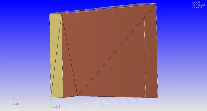
Now the above profile was of really high scaling, to reduce the number of grid points and meshing to be smooth and doable we have reduced to 0.001 scale. Thats how e perform Sub-Grid Scaling(SGS). Below is how we can change the scaling by using the transform tool.
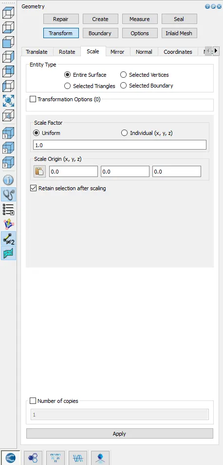
The main reason behind scaling to the lower scaled geometry is it decreases the number of cell counts making it easier to run simulation and mesh grid flow. The higher the sealed geometry the longer it takes for a simulation to cover running the whole flow.
Now that we have geometry set along with boundaries to be assigned as INLET, OUTLET, 2D WALLS, TOP, BOTTOM we can forward for the case setup now. Now the Assigning all types of Technical parameters for the flow property to case set up in the bottom right side. Below is the image is shown where all the case setup should like. The green tick indicates the all the parameter is set right according to flow properties. We can view this as below.
Assigning the boundaries is a must so that converge can recognize which is where to begin and understand the case setup part
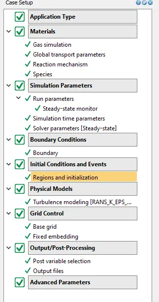
Before Jumping into the simulation part in Cygwin, one needs to set up the parameters in case set up to look like the above image. The value represents in the above image shows the completion of the properties, here's how every section needs to be done.
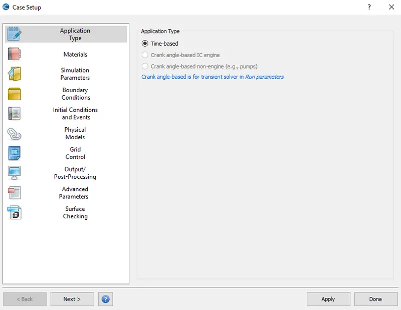
Application type:
Selecting the Time-Based is the option available here as we are only setting up a simple channel flow profile, to begin with.
Materials:
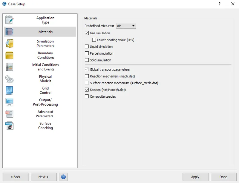
By selecting the predefined Mixture as AIR and checking Species.dat and gas simulation we complete materials setup.
Moving on to another section we have SPECIES where we O2 and N2 in the gas.
Moving on to Another section called Run Parameters where we assign very important terms to proceed.
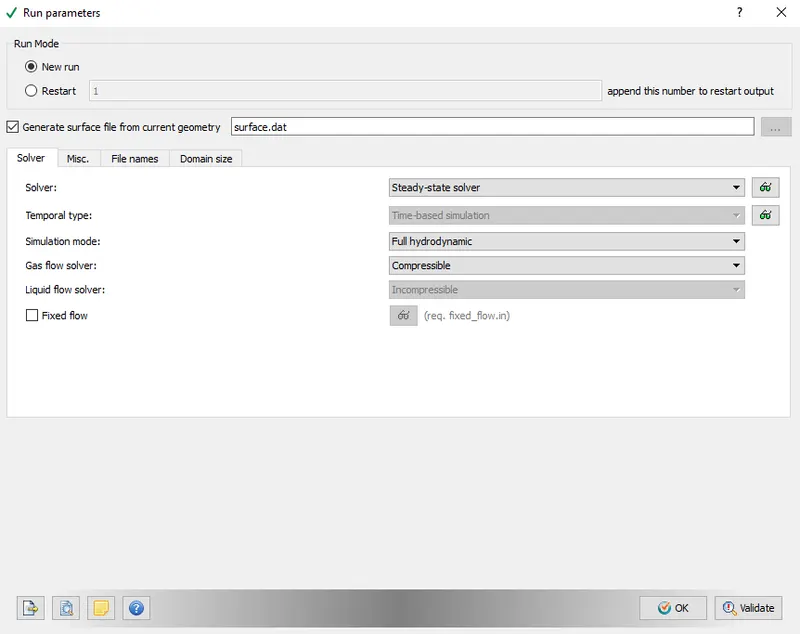
We select steady-state solver in the solver section and Full hydrodynamics in the solver section because we are going for simple channel flow. Where there is no complication in this system technically. The full hydrodynamic always take a lot of time to process the data files as it runs the basic Navier stokes equation through and through which might take a lot of time. Hydrodynamics would be a viable option here but again the fluid dynamics properties won't take place while running which is also not quite an option in some cases. SInce it's a simple flow Full hydrodynamics option can fully be considered and no complications would be three.
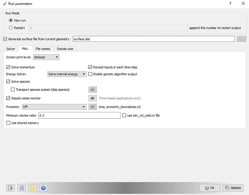
Followed by Solver we have the Misc. option where we select the steady-state here again including unchecking the used memory option as we don't want extra storage for the simulation.
Moving onto the steady-state monitor we have a list selecting section where we ADD first and then select Avg velocity. Now, this is the section where we need those parameters that we need to display when getting the output. So here we need to know the avg velocity of the flow when it flows out of the channel in OUTLET. That's is why assigning the value to the parameter.
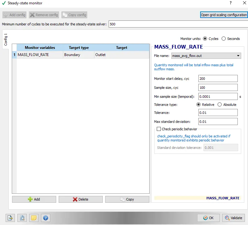
Assigning the value and validating it and Ok.
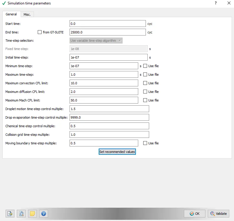
In another section called Simulation-Time Parametres here, we have all the values that are going to be involved in the simulation we are setting up.
The values here as follows for assigning. The end time is always 25000.
In the nest section of Solver-Parameters, we have what kind type of Navier-stokes solver, which is a Pressure-based solver for this flow.
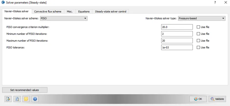
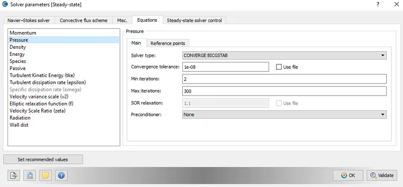
A slight change has to be made while we move further. In the EQUATION section, there are lot of Quantities in which PRESSURE has a default preconditioner value as SOR. WE have to make changes here to NONE because we don't need pressure values to be solved
The next section is really important as we assign the Boundary condition for the flow and the walls around it to define the type of fluid flow effect on it while flowing.
INLET - Region 0
OUTLET - Region 0
ELBOW-WALLS - Region 0
THROTTLEBODY- Region 0
above is how we assign the properties along with section-wise with INLET PRESSURE 150000.0 Pa and OUTLET PRESSURE 100000.0 Pa with 300K temperature in temperature boundary conditions.
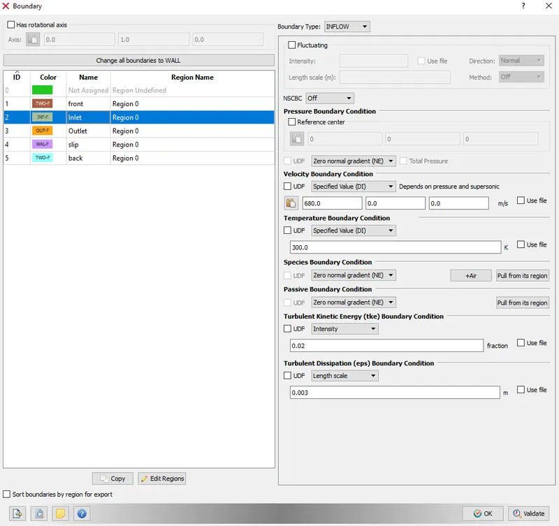
Here we adding nuemann boundary condition on OUTLET. Whats is NE neumann boundary condition?
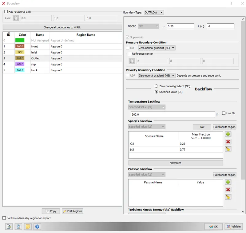
In the Region and Initialization, We need to add the O2 and N2 ratios for the flow. and We are adding velocity as an INITIAL CONDITION to the profile flow. VELOCITY here at first is 0ms the 680ms-1 and then 100ms-1 or different results with variation in flow properties.
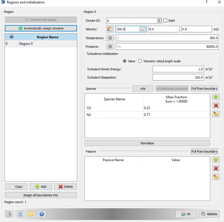
IN the Physical-Modelling We need to check the turbulence modeling as there will be turbulent flow over a channel because of the throttle body. We select the RNG k e method to solve the analysis.
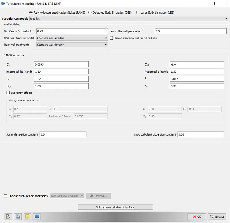
Now the next section is Base Grid, where we assign the INPUT coordinated for the channel so that it has a different output for different inputs. This where the box we create in the first stem gets its own assigned values of coordinates in a cartesian plane.
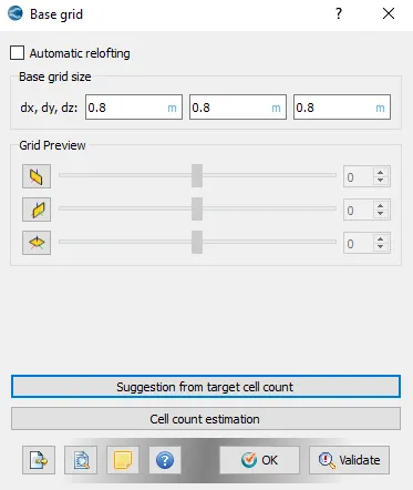
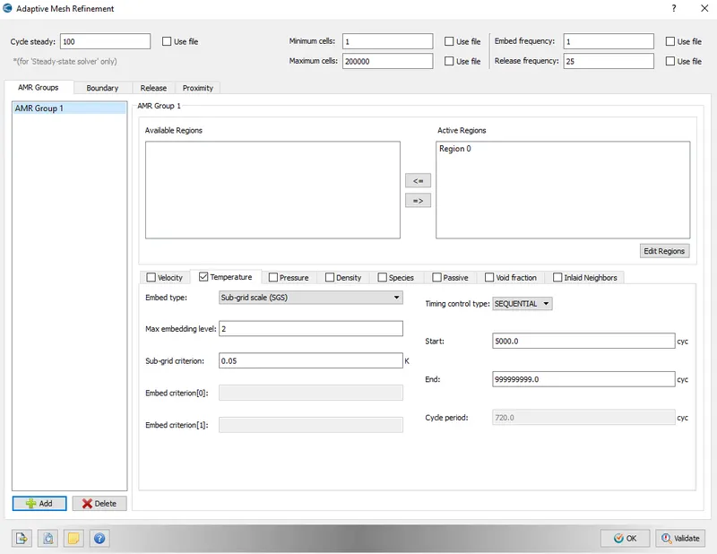
Now in this challenge we have a complex flow over a expansion fan where the sharp corner is present at the edge of fan. So for profile flow we need mesh refinement according to the change in temperature at a certain point so we can apply new section here called ADAPTIVE MESS REFINEMENT AMR which is in the GRID CONTROL section. here how we can allot values for the AMR.
Post-Process Simulation (CYGWIN):
Run Cygwin go to the directory where we have our basic .dat files in the converge folder. These are the following commands in Cygwin to go to the directory
$ cd
and tun the following command to convert,dat files into 3d OUtput dat files.
$ mpiexec.exe -n 2 "the path where you have intelmpi.exe" restricted </dev/null> logfile &

This was how-to convert .dat files into 3d Output data files for post-processing.
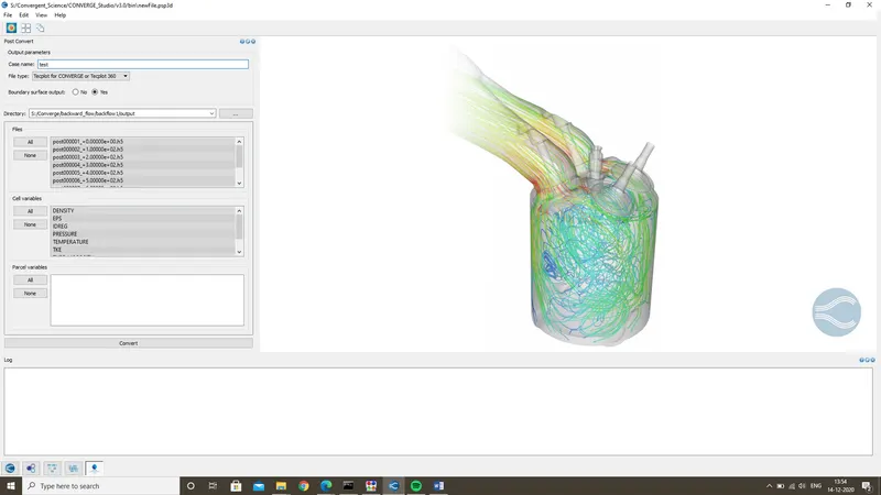
after that, we need to convert those files so that ParaView can read it 3d output files. We need to do through Cygwin to convert those files too with the following command or we can proceed with the converge itself as it provides nice feature to post convert 3D files to DAT files which Paraview can read. Here we need to name it as test and go to the directory of OUTPUT folder where all the files dumped and select ALL and CONVERT just like image shown below. and for post-processing the DAT and files we can directly convert it from CONVERGE as below.
OUPUT:
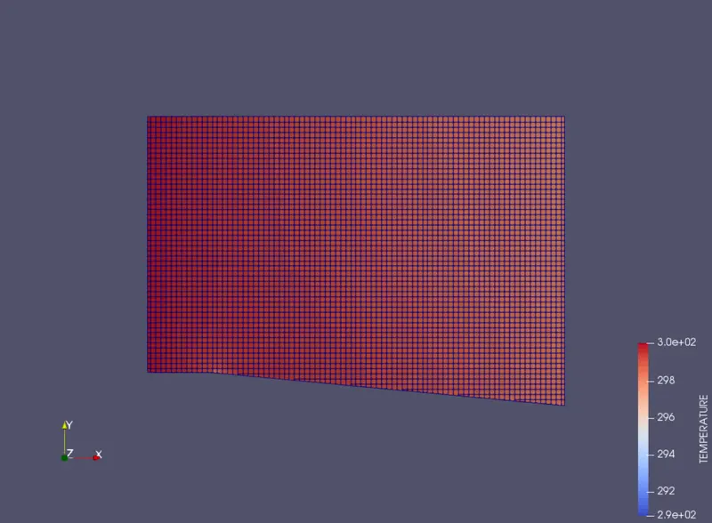
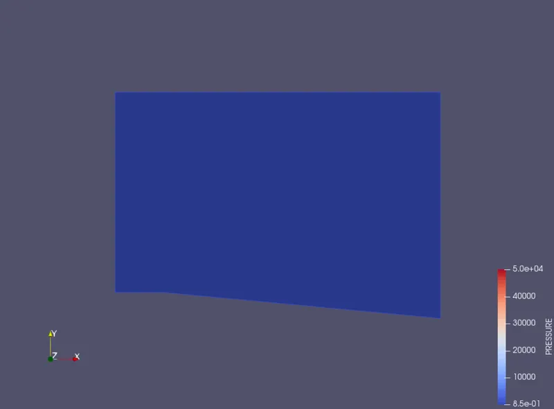
case 1: inlet velocity- 100ms-1 at 0.05K SGS (Sub-Grid Scaling)
Temperature contour:
Animation:
Pressure Contour:
Animation:
Case 2 : Inlet Velocity - 100ms1 at 0.01K SGS(Sub-Grid Scaling)
Temperature contour:
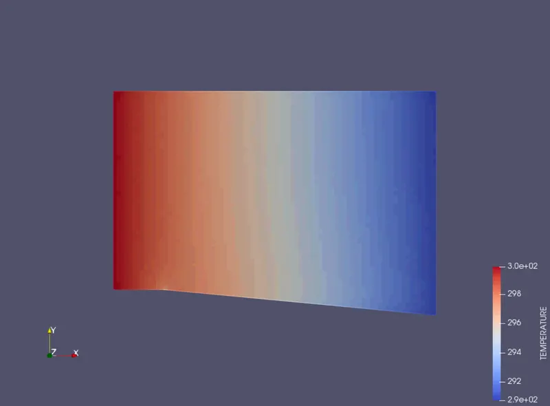
Animation:
Pressure Contour:
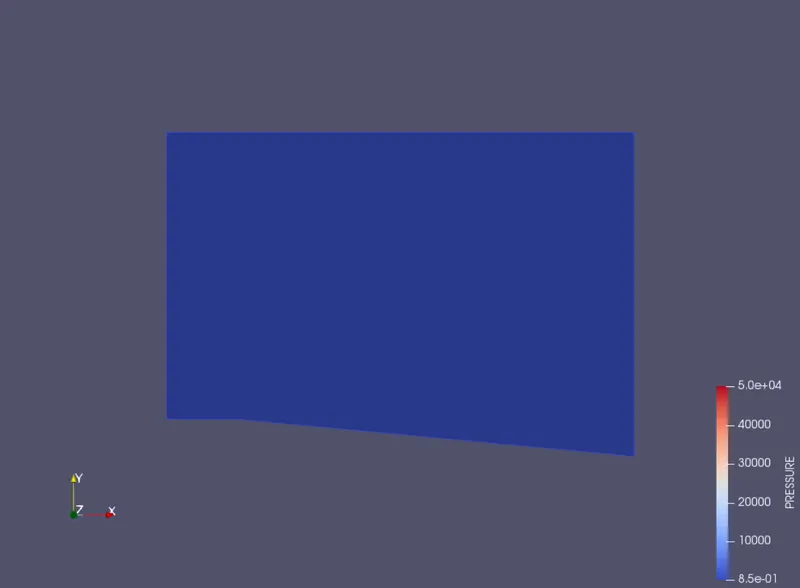
Animation:
Case 3: Inlet Velocity - 680ms-1 (supersonic) at 0.05K SGS(Sub-Grid Scaling)
Temperature contour:
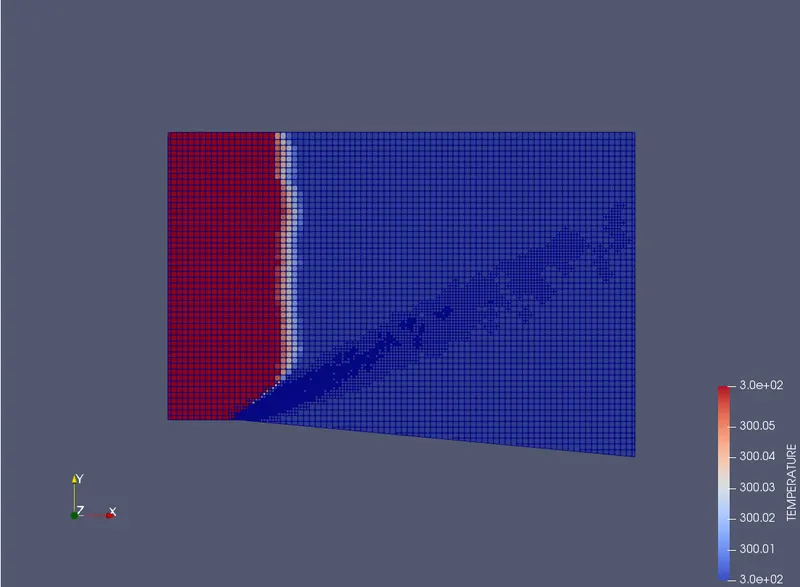
Animation:
Pressure contour:
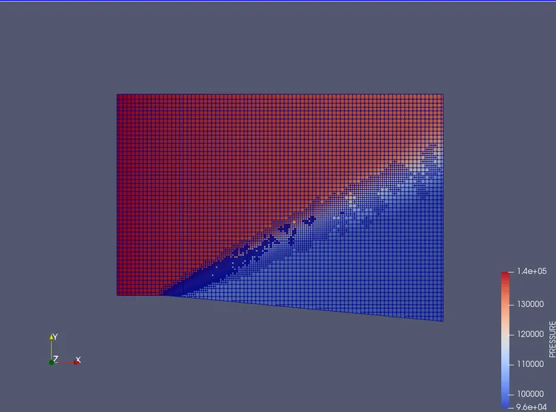
Animation:
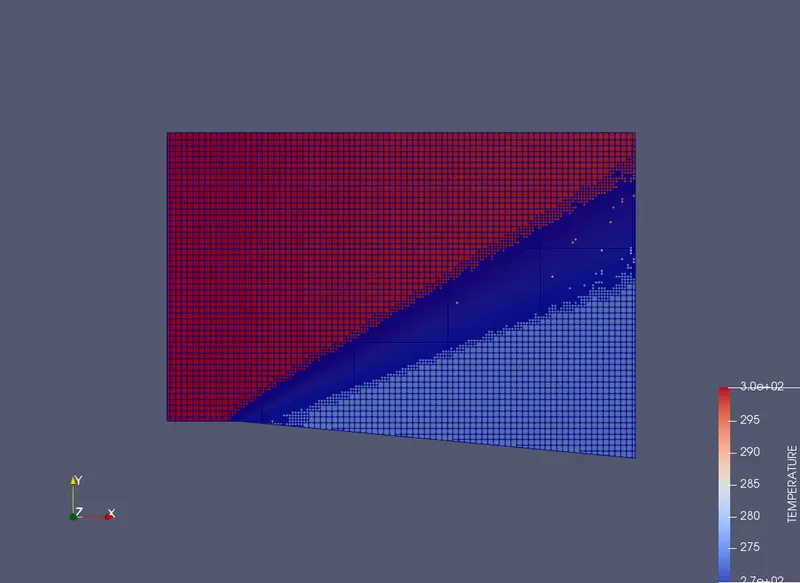
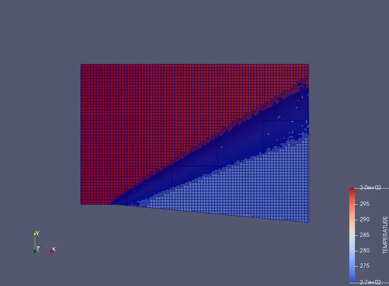
Case 4: inlet velocity - 680ms-1 at 0.01K SGS (Sub-Grid Scaling)
temperature contour:
Animation:
Pressure contour:
CONCLUSIONS:
As we had different outputs for different SGS and inlet velocity we can drive to a different conclusion such as:
1. With the lower inlet velocity the pressure, temperature, and mass flow rate increase but with the higher velocity, those all decrease.
2. with higher velocities the cell count increases taking a long time for simulation.
3. With recorded SGS and velocities when can calculate refined mach values at the shock distribution.
NOTE: As the SGS values are lower the mesh refinement is more compared to the previous values. It becomes refined more at the shock region. The reason being an increase in temperature converges refines substantially. At the inlet the velocity is supersonic but at the shock edge, it converts to subsonic where we can come to conclude as weak mach waves of expansion fan.
REFERENCES:
prandtlmeyerfan.DVI (caltech.edu)
What Are Boundary Conditions? Numerics Background | SimScale
Free boundary problems in shock reflection/diffraction and related transonic flow problems (nih.gov)