Week 5: Prandtl Meyer Shock problem

Aim

To simulate the Prandtl Meyer Shock Problem using converge CFD

1. Introduction and Theory

1.1 Shock wave

A shock is a type of propagating disturbance that moves faster than the local speed of sound in the medium. There is abrupt, nearly discontinuous, change in pressure, temperature, and density of the medium. A shock wave may be produced by supersonic aircraft, explosions, lightning or other phenomena that create violent changes in pressure.

1.2 Prandtl Meyer shock problem

Prandtl Meyer shock problem, also known as Prandtl Meyer expansion fan, occurs when a supersonic flow turns around a shard convex corner. It consists of infinite Mach waves diverging from the sharp corner, and these waves can be extrapolated to converge at the sharp corner. Each wave turns the supersonic flow in small steps. The velocity of the flow increases as it passes through the expansion fan and hence, the Mach number of the outlet flow is more than the inlet flow. However, there is a significant drop in pressure, temperature and density as the flow passes through the expansion fan.

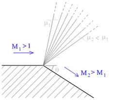
Fig 1: Prandtl Meyer expansion wave

1.3 Shock flow boundary conditions

In order to understand the significance of the shock flow boundary conditions, it is important to understand the different types of the boundary conditions. The most commonly used boundary conditions for a CFD case are Dirchlet boundary condition and Neumann boundary condition

1.3.1 Dirchlet boundary conditions

It is a type of boundary condition imposed on an ordinary or partial differential equations. It specifies the values of the differential equation that the solution must evaluate to, at the boundary of the domain.

For a differential equation such as:

y” + y = 0 in domain [a, b]

Dirchlet boundary conditions are: y(a)= a , y(b) = b

The predominantly used boundary conditions are velocity and pressure Dirchlet boundary conditions wherein, the inlet and outlet values for the characteristics are assigned during case setup.

1.3.2 Neumann boundary conditions

This form of boundary conditions also finds its application in ordinary and partial differential equations. However, unlike the Dirchlet boundary condition, when imposed on the equation, the boundary condition specifies the values for the derivative of equation at the boundary of the domain.

For a differential equation such as:

y” + y = 0 in domain [a, b]

Dirchlet boundary conditions are: y’(a)= a , y’(b) = b

1.3.3 Why Neumann boundary conditions are used for supersonic flows

In a supersonic flow, there is significant change in the characteristics of the fluid flow such as pressure drop, velocity increase, and temperature change and so on. This makes the definition of the outlet conditions at the boundary domain very difficult. A wrong value of the boundary conditions will result in the solution to blow up.

Hence, we make use of the Neumann conditions. In an ideal flow, there are two kinds of boundary characteristics that the flow has to satisfy,

• As there is no flow towards the wall (in a fully developed fluid flow), the component of the flow velocity normal to the wall is zero. It is also known as no-penetration boundary condition.
• Pressure boundary condition, which states that there cannot be a discontinuity in the static pressure inside the flow (since there are no shocks in the flow). In case of a fully developed flow, we can consider the pressure gradient at the outlet to be zero.

Thus, for a supersonic flow, the boundary conditions are as follows:

• Inlet: Velocity – Dirchlet BC, Temperature- Dirchlet BC (Mach number is dependent on this parameter), Pressure – Neumann (As the inlet boundary is already constrained with two Dirchlet BC)
• Outlet: Velocity- Neumann, Pressure- Neumann

2. Objective

To simulate the case of Prandtl Meyer shock wave and study the effect of SGS temperature on shock location and cell count.

3. Geometry

The computer aided model generated is imported into converge CFD. The model is scaled down using Transform command the boundaries are flagged as shown:

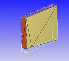
Fig 2: Geometry and boundary flags

4. Case setup

Application typeà Time-based

Materialsà Predefined mixture- Air & Gas simulation

Speciesà N2 & O2

Run parametersà Solver: Steady state solver

Simulation time parametersà Start time = 0 cycles, End time=25000 cycles; Time step: 1e-9 to 1 second; Max. CFL for convection =1.0

Boundary conditions:

Boundary	Type	Property
Inlet	Inflow	Pressure = NE, Velocity= 680 m/s , T= 286.1 K
Outlet	Outflow	Pressure = NE, Velocity = NE
Front 2D & Back 2D	2D	-
Top and Bottom	Wall	Slip (Viscous effects are negligible/Mesh grid size is more than boundary layer thickness)

Region creationà Assign all boundaries

Region initializationà O2 mass fraction=0.23, N2 mass fraction = 0.77

Physical modelà RNG k-Ɛ turbulence model

Grid controlà Adaptive mesh refinement

Base grid: dx= 0.8 m, dy= 0.8 m, dz= 0.8 m

AMRà Active region: Region 0, Maximum cells: 2 Lakhs, Embed type: Sub grid scale (SGS) , Max embedding level: 2, Sub-grid criterion: 0.05 K

Output filesà 3D output files: 1000 cycles, Restart output files: 1000 cycles

5. Results and discussion

5.1 Adaptive Mesh refinement

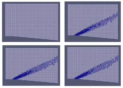
Fig 3: Mesh grid for different stages of simulation

As shown in the figure, the mesh grid is refined based on the temperature difference between successive grids defined by the sub-grid scale (SGS) parameter. AMR uses the second order derivative to refine mesh and is limited by the embedding level and the maximum cells allocated for simulation.

For a given base grid, the grid size can be calculated by using the formula:

Grid size = basegrid/ (2^(embed level)

5.2 Temperature, velocity and pressure contour

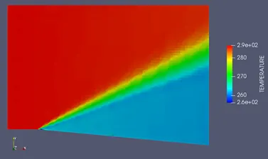
Fig 4: Temperature contour for case of velocity = 680 m/s and SGS = 0.05 K

Animation- Temperature contour

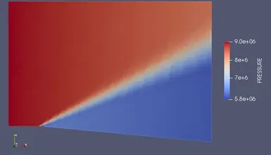
Fig 5: Pressure contour for case of velocity = 680 m/s and SGS = 0.05 K

It can be seen from the contour plots that there is a significant drop in pressure and temperature as the fluid flows through the expansion fan. Another observation from these contour plots is the origin of the expansion fan from a point source. This point source is coincident with the sharp corner from which the expansion waves diverge.

On the other hand, the velocity of fluid flow is found to increase. This velocity increase can also be validated by plotting the Mach number for the inlet and outlet.

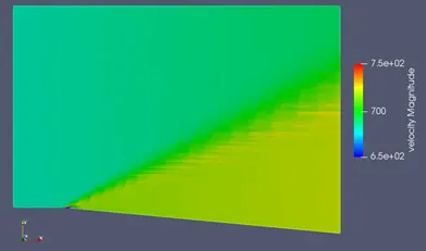
Fig 6: Velocity contour for case of velocity = 680 m/s and SGS = 0.05 K

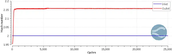
Fig 7: Mach number plot

5.2 Effect of SGS temperature on shock location and cell count

To study the effect sub-grid scale, we simulate the case with additional SGS values. In this section, the results are compared for the SGS values of 0.05 K, 0.1 K and 0.3 K

5.2.1 Effect on shock location

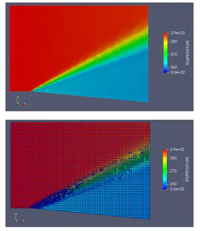
Fig 8 Temperature plot for SGS=0.05 K

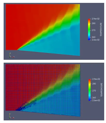
Fig 9: Temperature contour plot for SGS=0.1 K

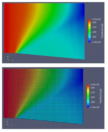
Fig 10: Temperature contour plot for SGS=0.3 K

As there is an increase in SGS parameter, we see that the expansion fan becomes broader with a blurred origin point as opposed to a sharp corner with narrom expansion fan obtained with smaller values of SGS. At higher values of SGS, there is no adaptive mesh refinement as the criterion is never found to be true.

5.2.2 Effect on cell count

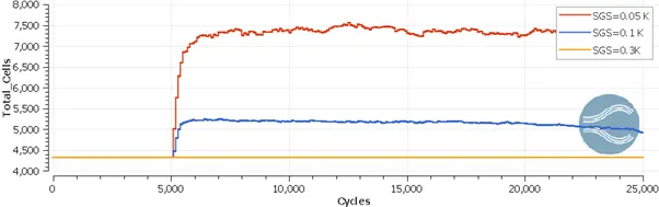
Fig 11: Total cell count for the three cases

We can see that as the SGS parameter is reduced, there is a significant increase in the cell count. Hence, more accurate results, the expenditure of simulation is bound to increase.

6. Conclusion

Thus, the case of Prandtl Meyer shock problem is successfully simulated using converge CFD.