Prandtl Meyer Shock problem

Prandtl Meyer Shock Flow

Aim: To simulate Prandtl Meyer Shock flow using Converge.

Objective:

• To Setup and run the case on Prandtl Meyer shock flow for supersonic inlet condition.(velocity=680m/s)
• To Setup and run case on Prandtl Meyer shock flow for subsonic inlet condition.(velocity=100/s)
• Post process and compare results for both the cases.

Description:

Prandtl Meyer expansion fan is a two dimensional simple wave. It is a centered expansion process that occurs when a supersonic flow turns around a convex corner. The fan consists of a finite number of Mach waves diverging from a sharp corners. When a flow turnsaround a smooth and circular corners, these waves can be extended backwards to meet a point.

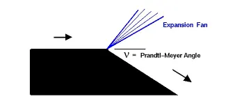
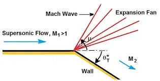
Each wave in the expansion fan turns the flow gradually. Near the expansion fan,the flow accelerates and the Mach number increases, while the static pressure , temperature and density decreases. As the process is isentropic process, the total temperature, total pressure remains constant across the fan.

ShockWaves:

• Shock wave is a type of propagating disturbance that moves faster than the local speed of sound in the medium.
• Shock wave is a very thin region in a flow where supersonic flow is declerated to subsonic flow. The process is adiabatic but non-isentropic.
• Across the shock there is always an extremely rapid raise in pressure, temperature and density of the flow.
• Shock waveare characterized by an abrupt nearly discontinuous change in characteristics of the medium.
• Shock wave is a very thin region in a flow where supersonic flow is decelerated to subsonic flow.
• Shock wave is not conventional sound wave.
• It travels through most media at a higher speed than an ordinary wave. When a shock wave passes through matter the total energy is preserved.
• A shock wave is a large compressibility wave and takes the form of a very sharp change in the gas properties.

Mach Number(Ma) - The ratio of the speed of a moving object to the speed of sound ina fluid is known as the Mach Number. Speeds less than the speed of sound have a Mach number between 0 & 1, these are called as Subsonic. Speeds which are greater than the speed of sound have a Mach number greater than 1 are called as the supersonic.

Formation of Shock Wave:

a. Mach Number is less than 1, that means subsonic flow.

b. Mach Number is equal to 1, that means sonic flow.

c. Mach Number is greater than 1, that means supersonic flow.

Ma=V/C where, Ma=Mach Number

V= velocity of fluid/body moving

C= velocity of sound in fluid

Types of Shock Wave:

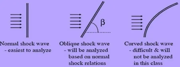
a. Normal Shock Wave - If the shock wave is perpendicular to the floe direction it is called a normal shock. A normal shock occurs in front of a supersonic object if the flow is turned by a large amount and the shock cannot retain attached to the body.

b. Oblique Shock - An oblique shock wave is one that is not perpendicular to the direction of the fluid flow. Such a shock wave arises when a fluid stream flowing at a supersonic speed moves along a convergent or divergent boundary.

c. Bow/curved shocks - When an oblique shock is likely to form at an angle which cannot remain on the surface, a nonlinear phenomenon arises where the shock wave will form a continuous pattern around the body. In these cases, the 1D flow model is not valid and further analysis is needed to predict the pressure forces which are exerted on the surface.

Types of Boundary Conditions:

• Dirichlet Boundary Condition
• Neumann Boundary Condition
• Robin Boundary Condition
• Mixed Boundary Condition
• Cauchy Boundary Condition

• Dirichlet Boundary Condition- This boundary condition specifies the value of variable at a boundary. It may also be called a fixed condition. Hence itis used when a value needs to be imposed at a boundary.
• Neumann Boundary Condition- This boundary condition specifies the derivatie of a variable at a boundary. It is used rather than the actual value when a certain rate of change in vakue needs to be imposed for a variable.
• Robin Boundary Condition- It is alinear combination of Drichlet and Neumann boundary condition applied to the entire boundary. Robin conditions are used to mdel Newton's law of cooling , where heat flux is praportional to temperature.
• Mixed Boundary Condition- The different types of boundary conditions in different parts of the boundary. While in the Robin BC, single constraint consisting of different BC applied to complete part of a boundary.
• Cauchy Boundary Condition- Here both Drichlet and Neumann BC i.e two constraints are applied to complete boundary.

Procedure:

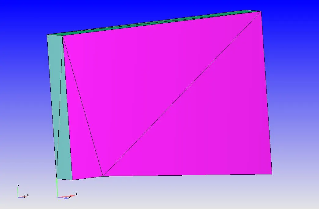
• Initially open Converge Studio and import the geometry.
• After setting the geometry, next important thing is to diagnosis the geometry for errors/problems. For this go to Right Bottom side, select Diagnosis > click on All intersections > click Find. On top we can check for problems in Problem Triangles.
• Now if there are no errors found then the geometry is correct.
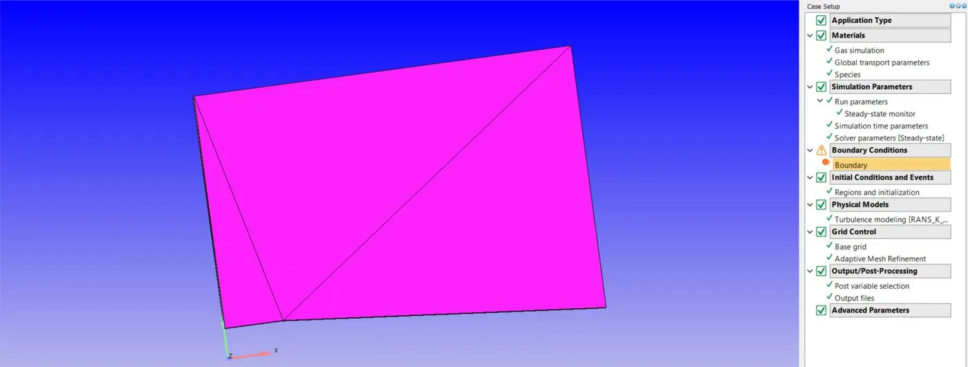
• To we should do Case Setup. Just beside Diagonisis > click on Cae Setup > in case setup window we can see 'Begin Case Setup" > click on it to set the setup.

Case Setup-

Application Type = Time-based

Materials -

Predefined mixtures = Air

Select 'Gas Simulation' and 'Reaction Mechanism'

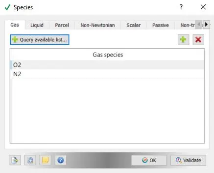
> Click on Species > select Gas > click on Add and select N2 &O2.

Simulation Parameters-

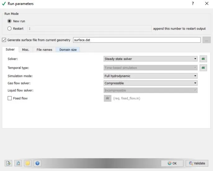
In Run Parameters two main things to be considered:-

(a.) select the following solver settings

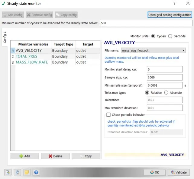
Steady State Monitor:

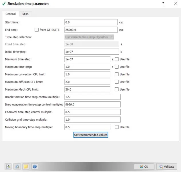
Simulation Time Parameters-

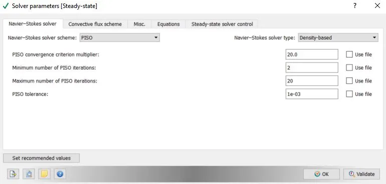
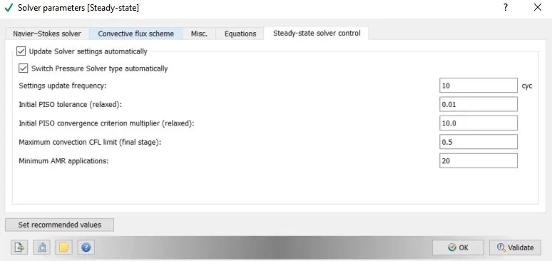
Solver Parameters [Steady-State]-

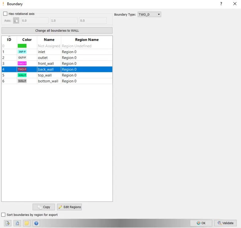
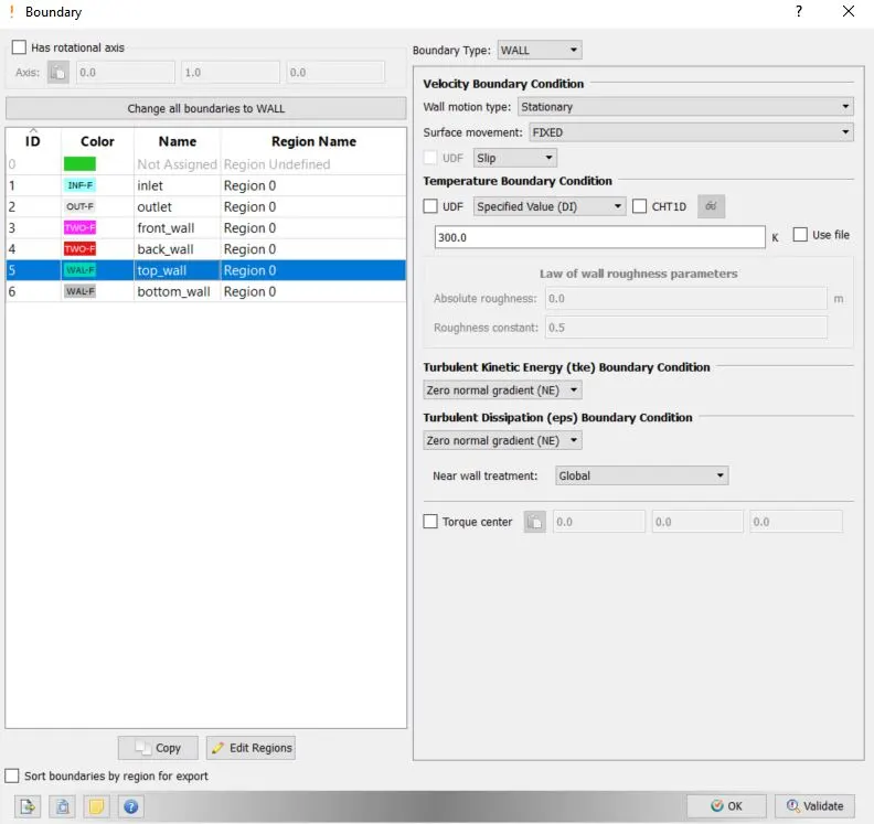
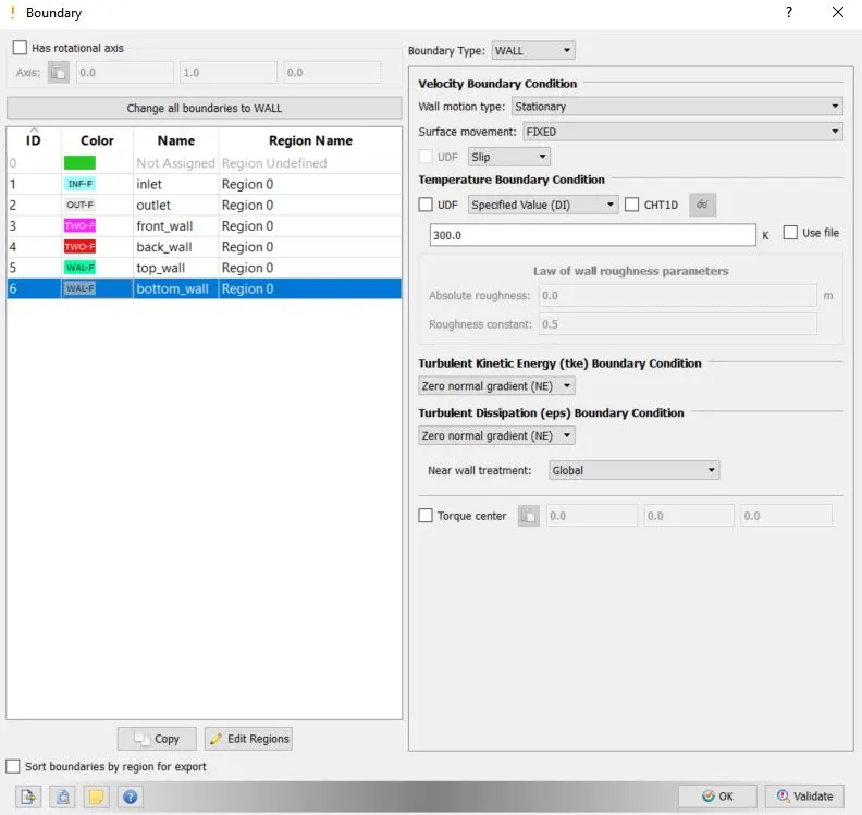
Boundary Conditions-

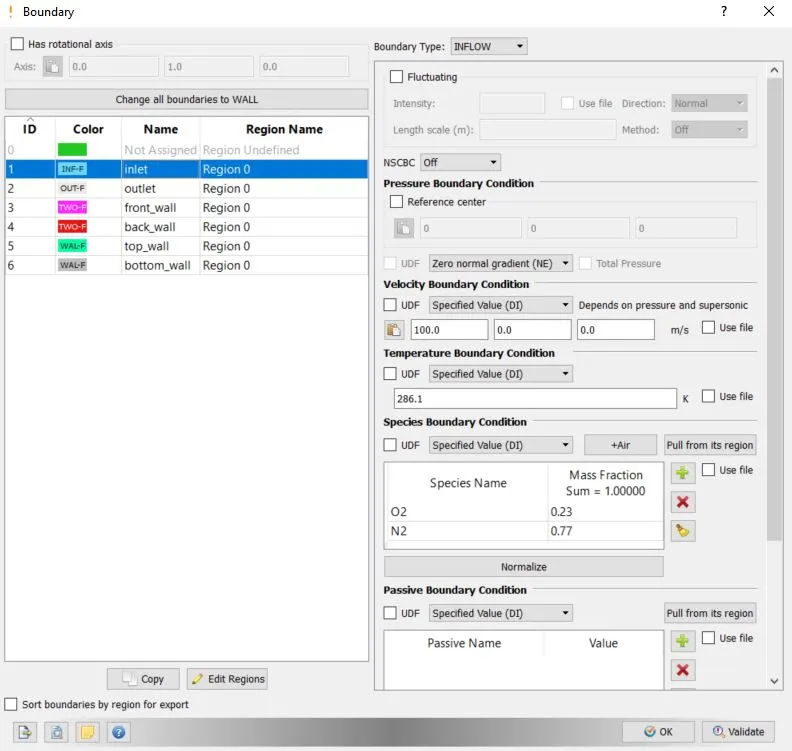
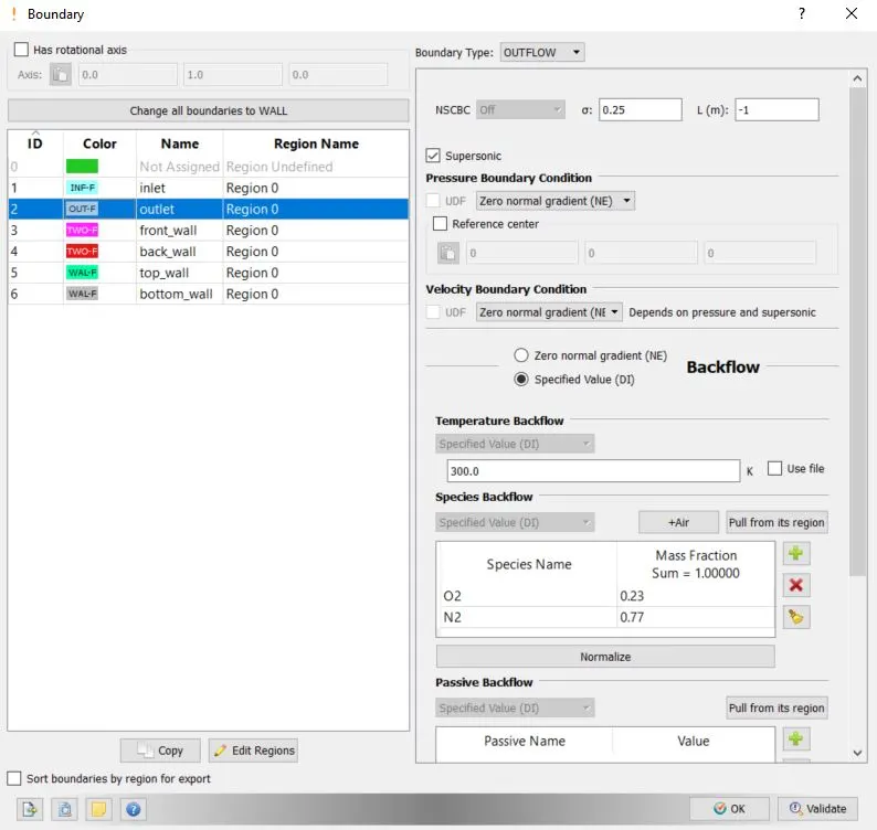
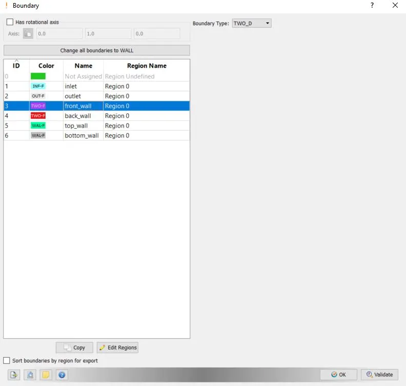
Booundary:

Initial Conditions and Events:-

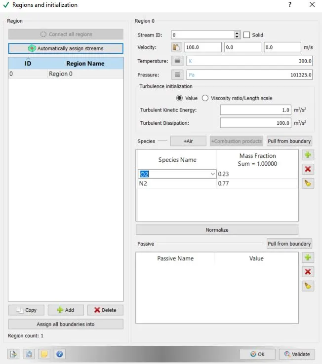
Regions and Initialization:

Physical Models:-

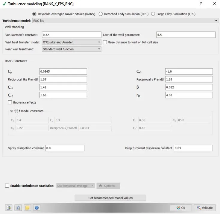
Click on Physical Models and select Turbulence Modeling in this case.

Turbulence modeling-

Grid Control:-

Now click on Grid Control > select Adaptive Mesh Refinement

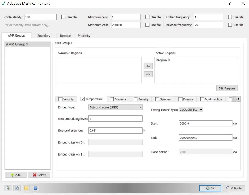
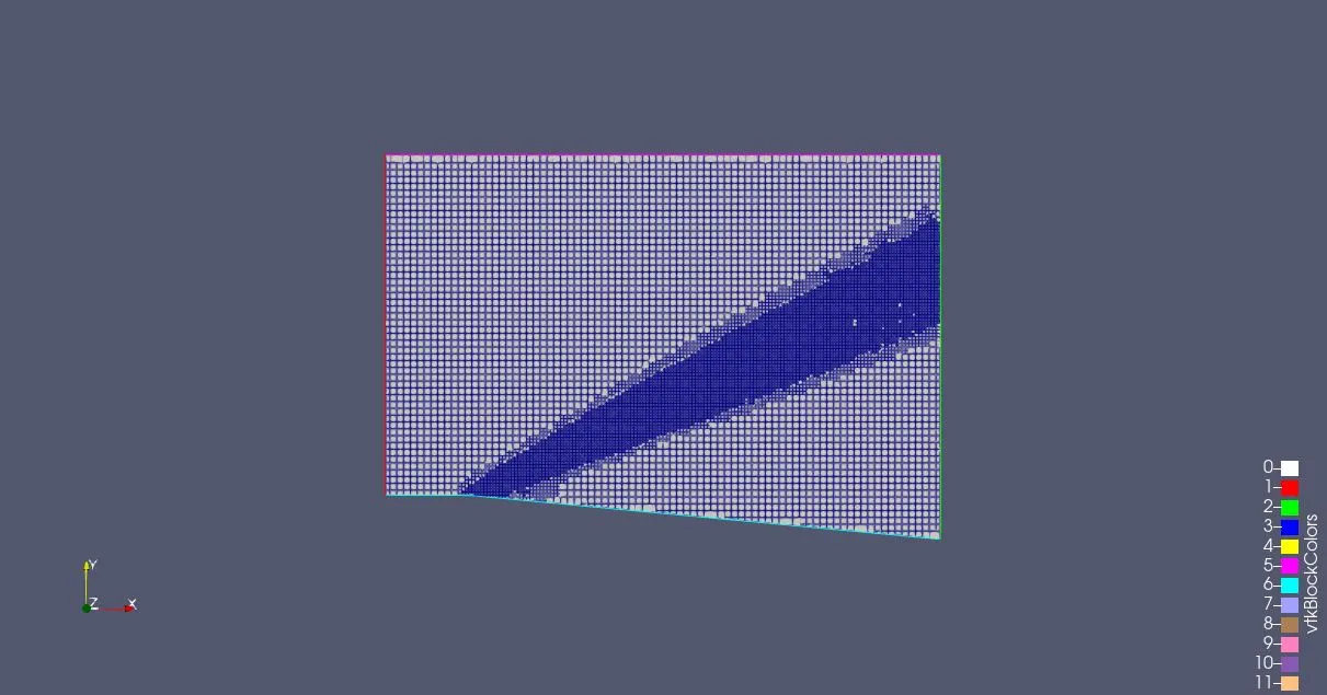
• Here the Sub-grid criterion value is changed as per the case we are simulating (0.05, 0.03 and 0.01).

Post-Processing:-

Post Variable Selection:

Click on Typical Variables/Geometry > Select required variables.

Output Files:

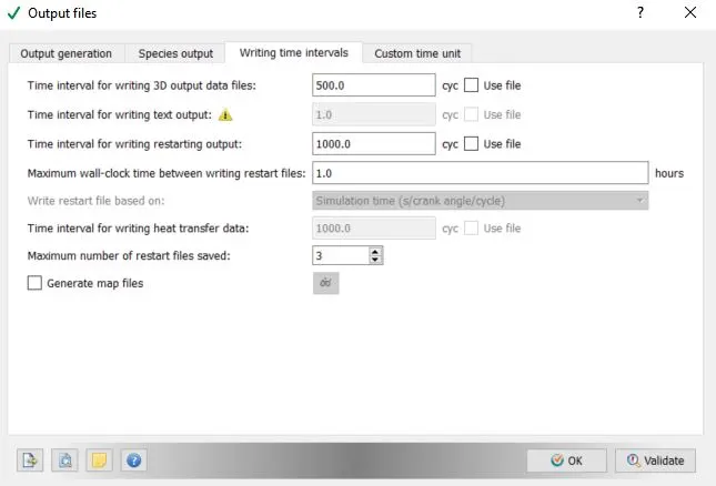
• With this setting up of the case is completed.
• Now go to File > Export > click on Export Input Files. select the destination folder(test) to save the data.

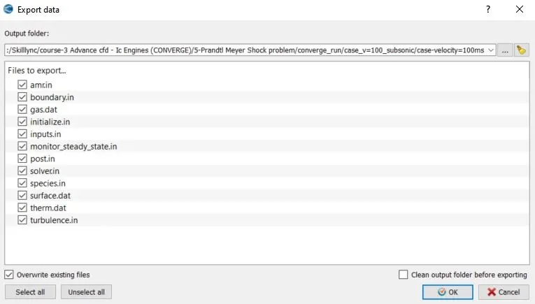
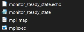
• After importing the input files, paste the "mpiexec.exe file".

• Now open Cygwin and navigate to the location where the setup files are imported.

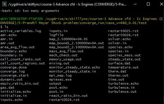
• Once we navigate to the respective folder, we need to run the simulation. To run the simulation use the following command in Cygwin;

>> Here path is copied from " C:ProgramFilesConvergent_ScienceCONVERGE3.0.15binconverge-intelmpi.exe ".

• Now the simulation starts running , and it displays the steps in cygwin. As the simulation begins it creates multiple folders (i.e. '.scratch' & output) in the path where we saved the input files.

• Once the simulation is complete, to perform post processing we need to convert the obtained result data into format where we can access in Paraview. These converted files are directed to the Output folder.

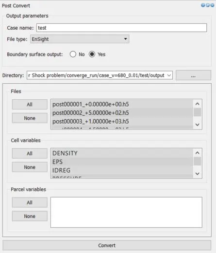
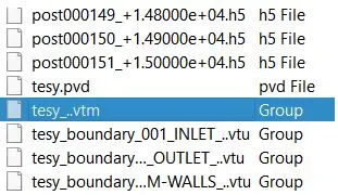
• Open PARAVIEW > direct to folder where the output is saved > select '.vtm(group file)' > data imported to paraview.

• Necessary contours, profiles and animations are generated using paraview. To generate plots we can use ConvergeStudio (line plotting option).
• Hence required plots, contours , animations are obtained in order to study the results.

Geometry:

Case Setup:

Observations:

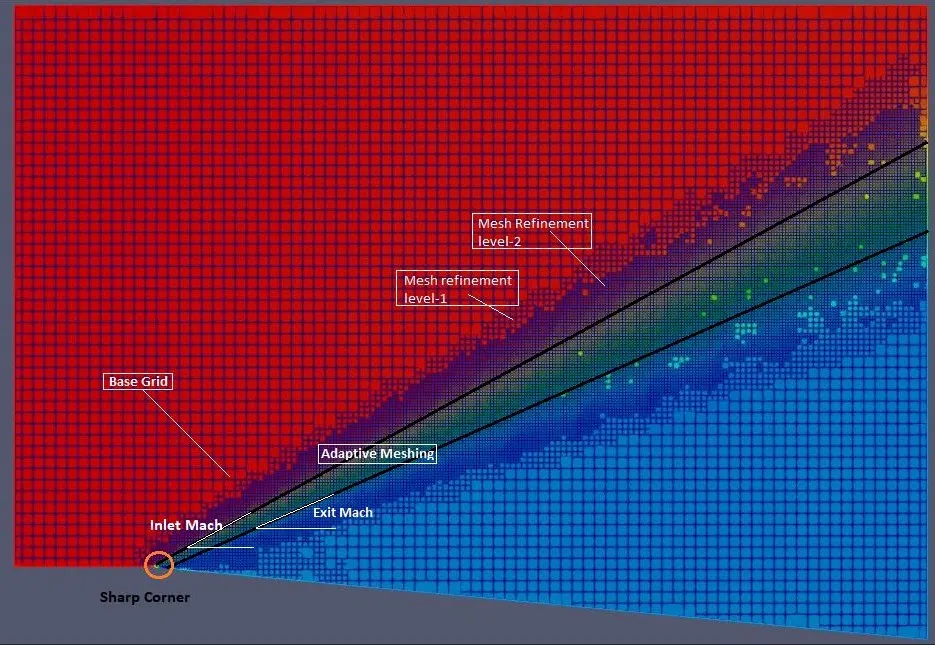
Prandtl Meyer shock flow for supersonic inlet condition

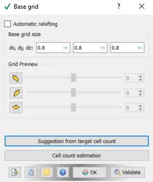
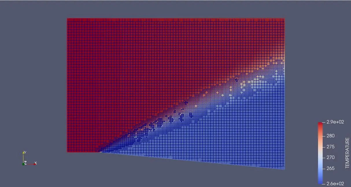
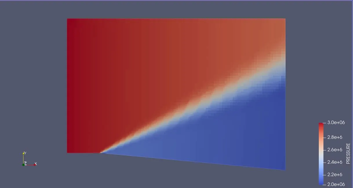
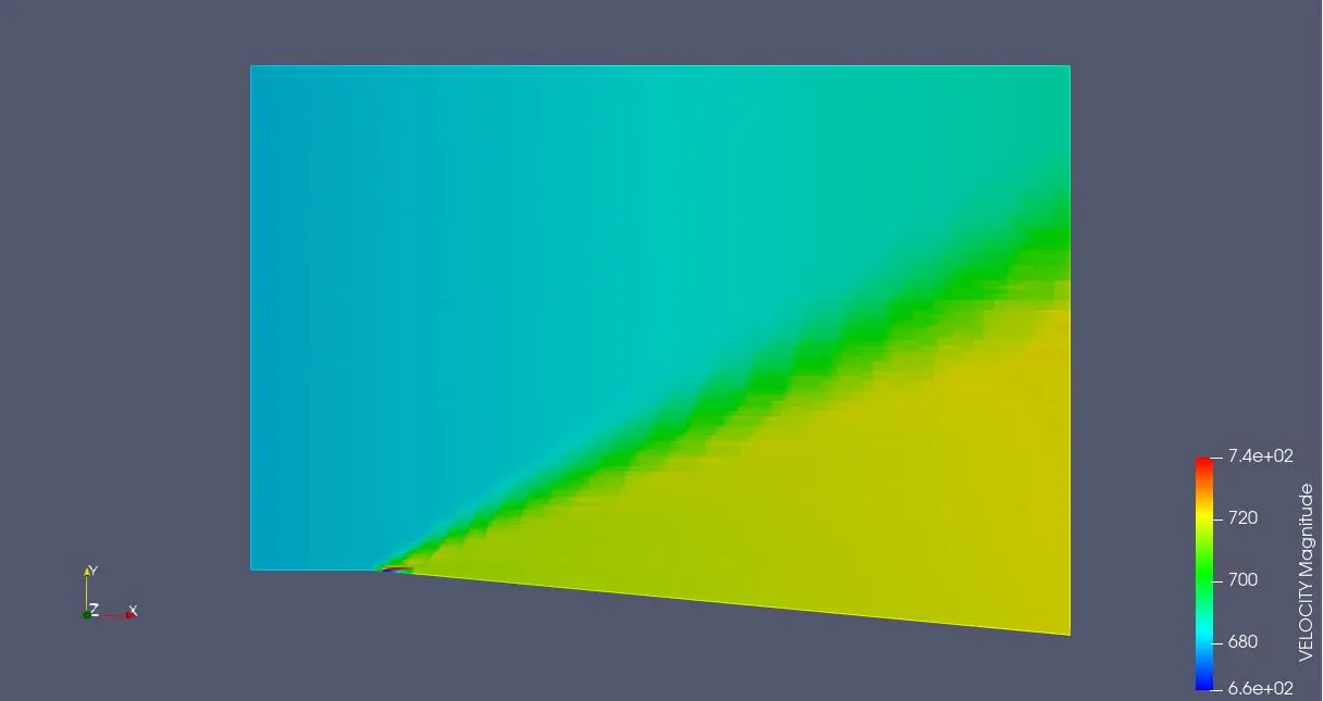
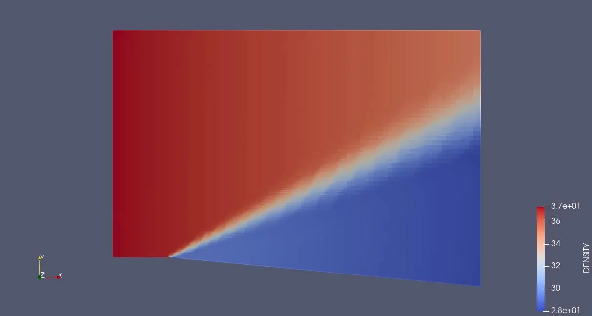
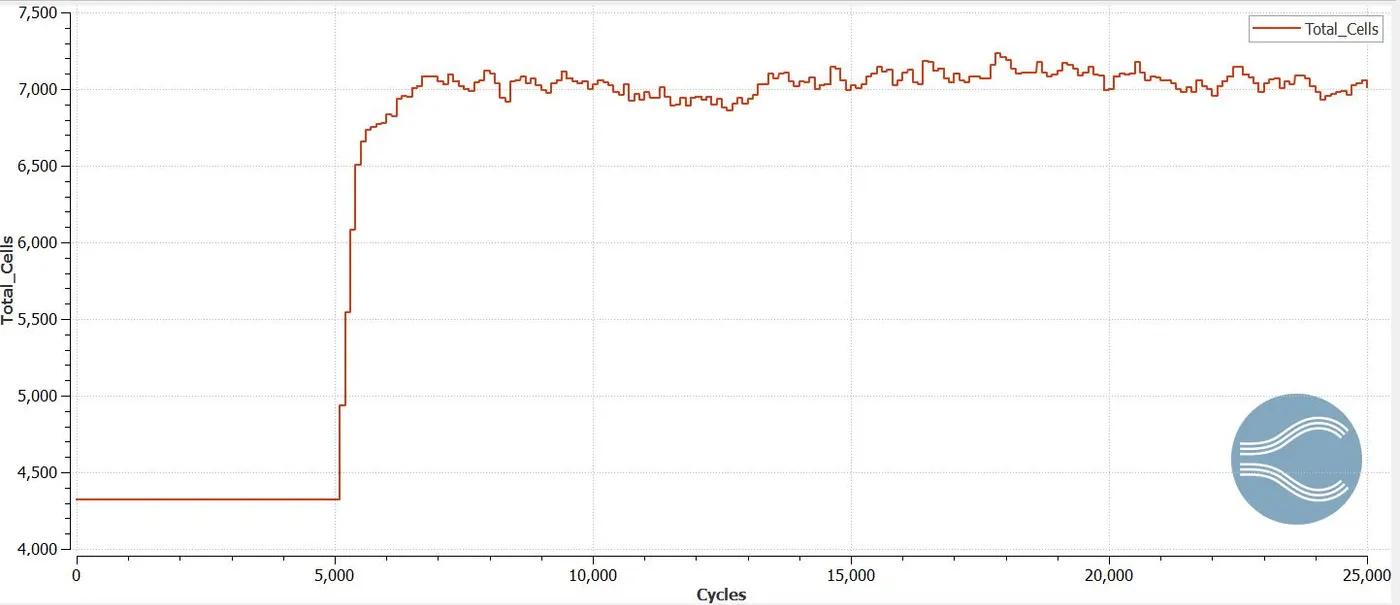
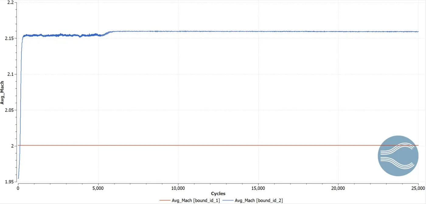
Case-1 Velocity=680m/s, Sub-Grid Scale Temperature(SGS)=0.05K and Base grid = 0.08m.

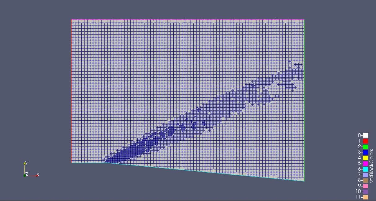
Temperature Contour:

Pressure Contour:

Velocity Contour:

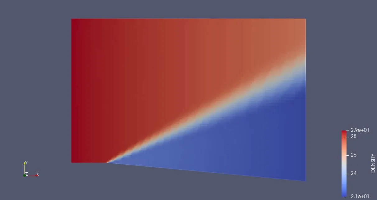
Density Contour:

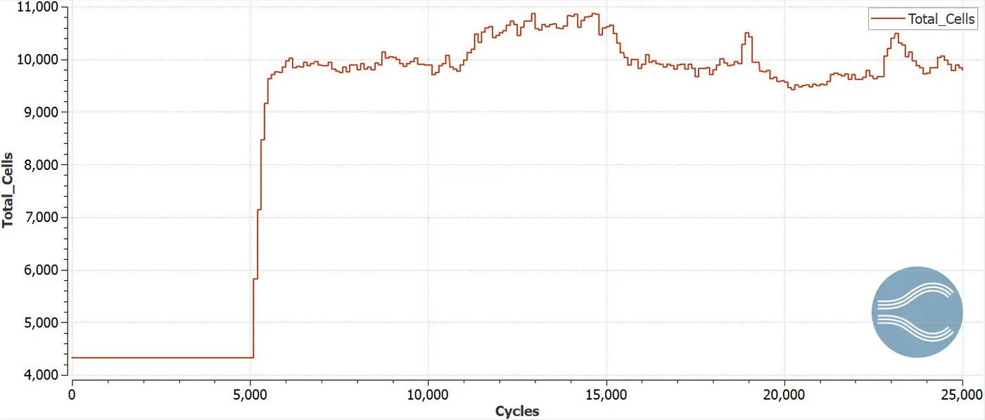
Cell Count:

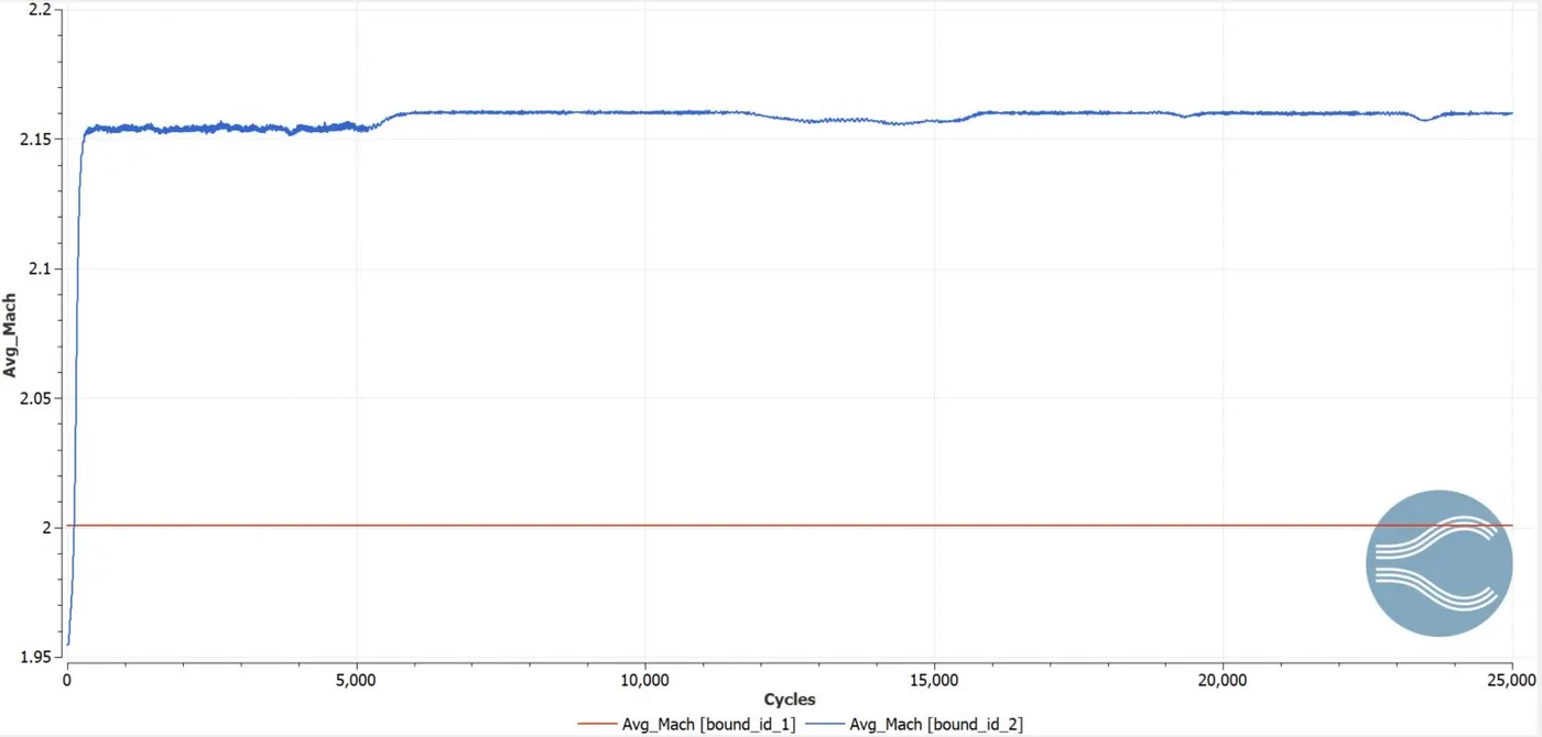
Mach Number plot:

Animation:

Case-2 Velocity=680m/s, Sub-Grid Scale Temperature(SGS)=0.03K and Base grid = 0.08m.

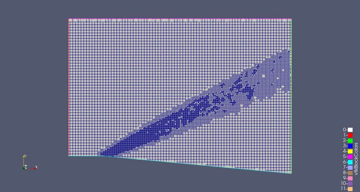
Temperature Contour:

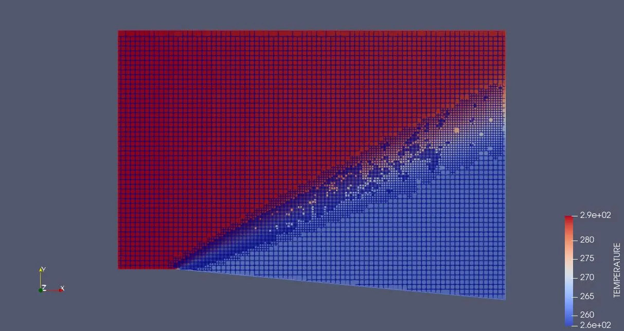
Pressure Contour:

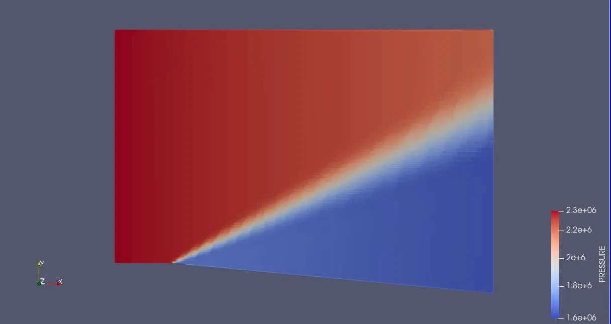
Velocity Contour:

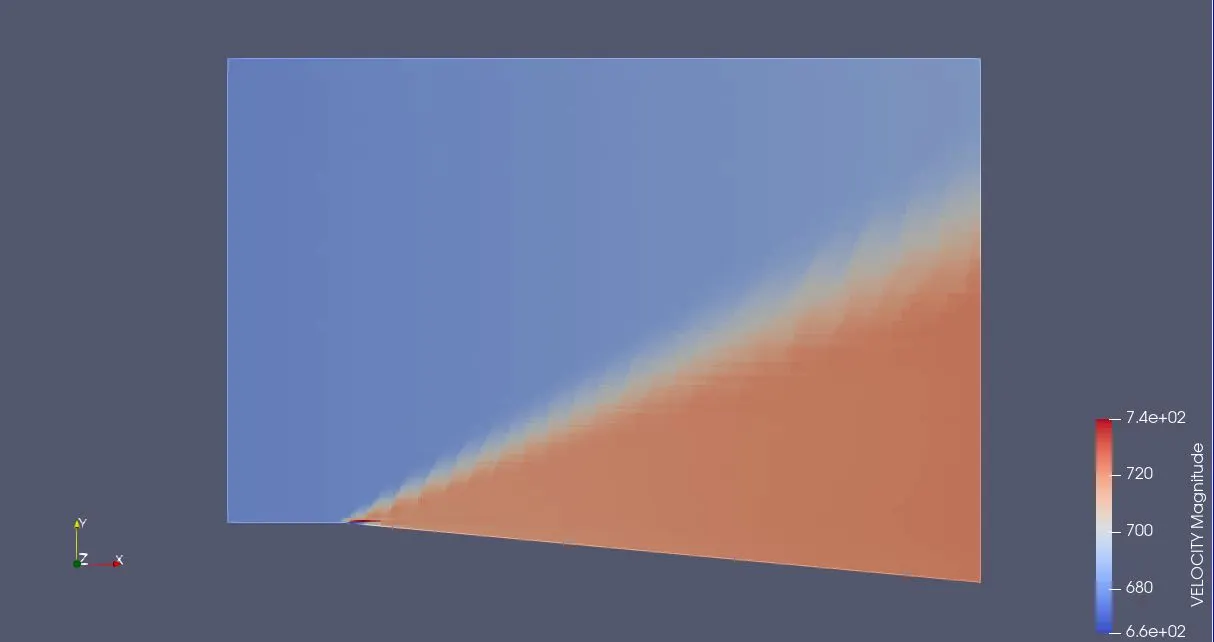
Density Contour:

Cell Count:

Mach Number plot:

Animation:

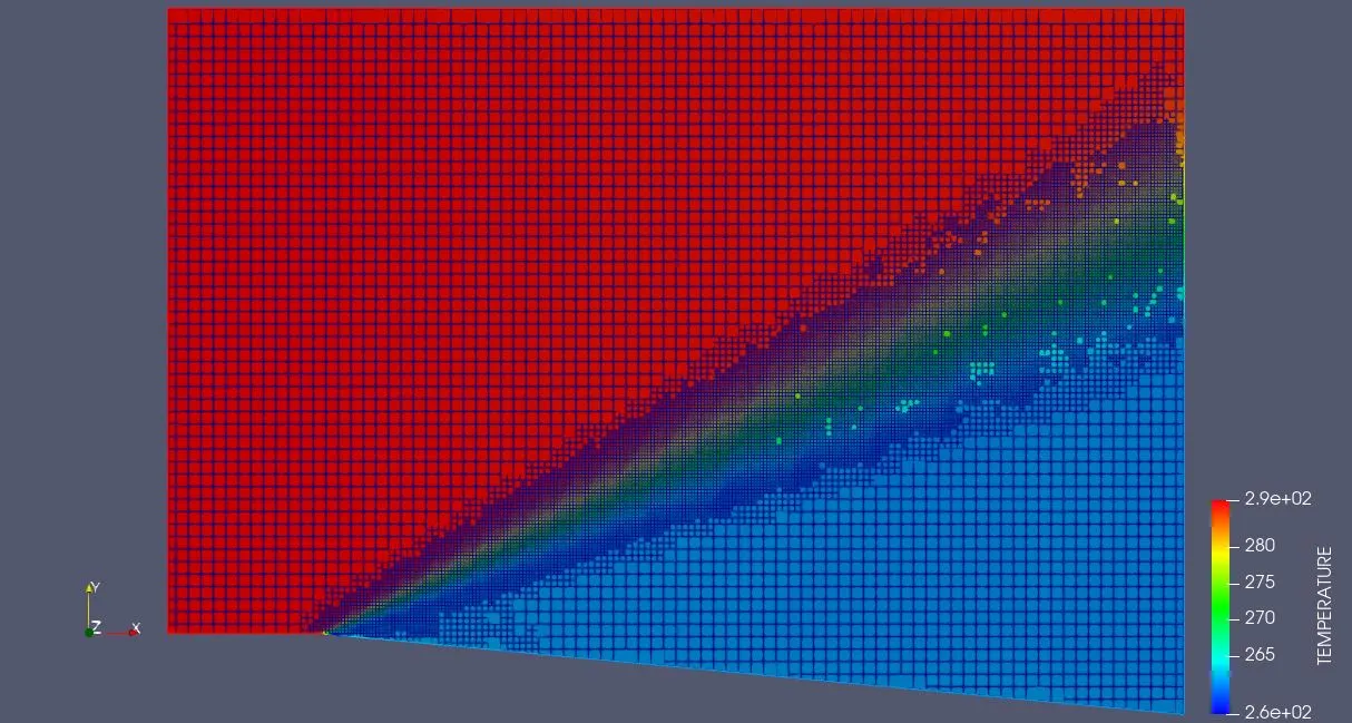
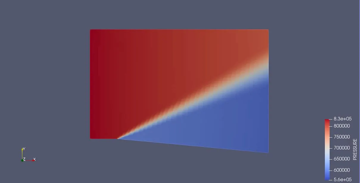
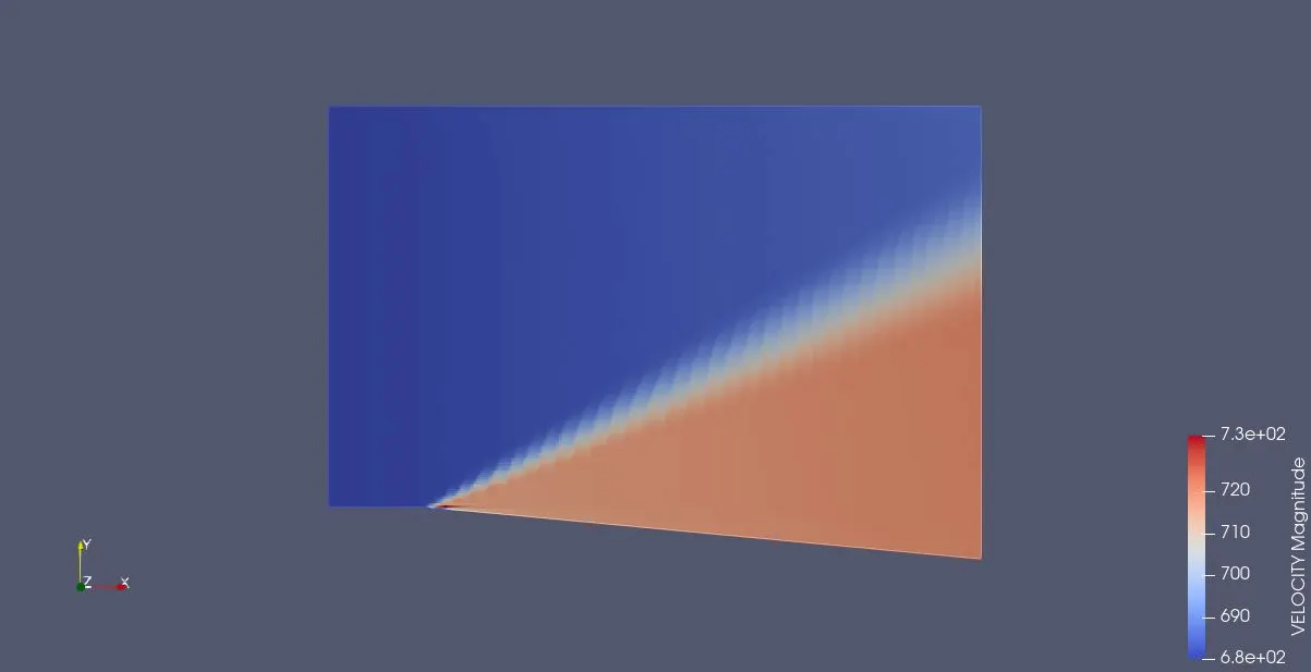
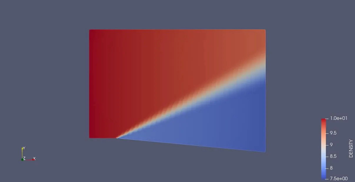
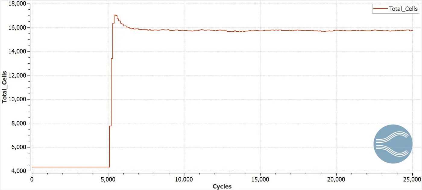
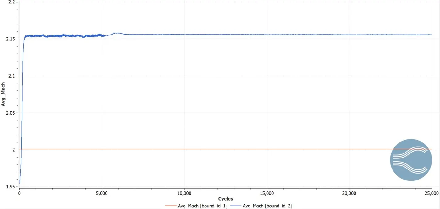
Case-3 Velocity=680m/s, Sub-Grid Scale Temperature(SGS)=0.01K and Base grid = 0.08m.

Temperature Contour:

Pressure Contour:

Velocity Contour:

Density Contour:

Cell Count:

Mach Number plot:

Animation:

Prandtl Meyer shock flow for subsonic inlet condition

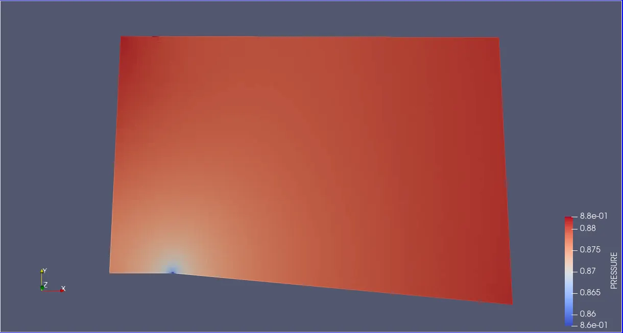
Case: Velocity=100m/s

When the inlet velocity of the flow is subsonic, there wont be any shock wave produced as we can see in supersonic flow. Here as this is a initial phase there is no developement of shock wave.In supersonic flow we can clearly identity the point where the shock flow starts. Hence they donot show any similar results as compared to the supersonic flow.

Animation:

Results:

• The effect of sub-grid scale on cell count has been observed based on the temperature i.e. 0.05,0.03,0.01. From the obtain contours, it can be observed that the sub-grid scale based on the temperature is decreased- the cell count increases as the AMR gets activated.
• From the contours, the place where the shock occurs there we can see the finer cells. This is called as Adaptive Mesh Refinement.
• The effect on a mesh can be observed in the Prandtl-Meyer shock generation region as the AMR algorithm gets activated for different sub-grid scale temperature(monitered temperature in curvature)
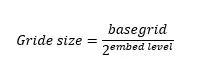
• On increasing the embeded scale, it is observed that the cell size becomes smaller.
• Leading edge that the shock wave makes is praportional to the inlet Mach Number and the trailing edge of the shock depends on the out flow Mach Number.
• Due to the Prandtl Meyer shock flow , the flow undergoes an abrupt change in reduced flow properties such as density, pressure and temperature across the expansion fan.
• For a subsonic case i.e. velocity=100m/s, the flow doesn't get expanded at the sharp corner and hence there is no expansion fan observed. But clearly we can see the point where the shock wave starts.

Conclusion:

• Simulations for both subsonic and supersonic are performed in order to compare the result and understand how the at the effect of SGS temperature value on cell count and the shock location.
• From the simulation it is observed how the Adaptive Mesh Refinement is an important tool to capture the shockwave effectively using a sub-grid criterion based on the curvature of a parameters like veocity and temperature.
• The effect of SGS parameter on shock location is also recorded.
• The theoratical study helped in selecting the right boundary conditions that are used for shock flow problems.
• Various contours, plots and animations are generated in order to have clear understanding.