Week 5: Prandtl Meyer Shock problem
Prandtl Meyer Shock Wave Simulation
Objectives:
Simulate the Prandtl Meyer Expansion Shock and investigate the effect of SGS parameters on shock location and temperature.
Waves in Compressible flow:
- Gas flow over a body creates a disturbance that propagates through the fluid domain and interacts with other parts of the body. These disturbances are called waves and their motion is referred to as wave motion.
- Two features of Compressible waves are shock waves and expansion waves.
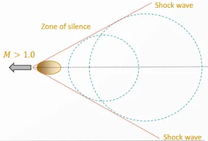
- A shock wave is a fluid flow disturbance propagating through the gas faster than the local speed of sound. As the object moves through the fluid at a supersonic speed, waves generated by its motion cannot propagate upstream. Instead, they coalesce a short distance in front of the object, forming a very thin wavefront called a shock wave.
- The lag of the wavefront behind the object restricts them to a cone-shaped region. Wavefront at the edge of this cone forms a shock wave which is effectively the downstream part of the upstream shock.
- The shock that is oriented perpendicular to the flow direction is called a normal shock. If they are inclined at an angle to the flow, they are called oblique shocks. A shock that is displaced upstream away from the impingement point of the body and arcs away from this position as an oblique shock is called a bow shock.
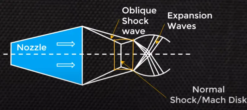
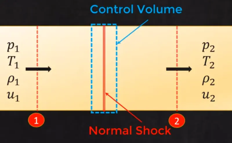
- Shock waves are very thin on the order of magnitude of the mean free molecule path. Thus in the continuum description of gas dynamics, they are treated as discontinuities. Shock waves are characterized by an abrupt change of flow properties such as an increase in static properties such as pressure, temperature, density, and a decrease in Mach number and total pressure, also an increase in entropy.
Expansion waves:
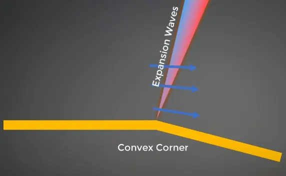
- Expansion waves/fan is another type of wave in supersonic flows. They develop when the flow area suddenly expands i.e., supersonic flow meets a convex corner. They deflect away from their own flow path leading to an expansion fan causing an abrupt change in properties such as an increase in Mach number and decrease in static flow properties on contrary to the shock waves.
- The expansion region is continuous in that the properties vary relatively smoothly which is opposite to the abrupt change across a shock as shown in the below figures.
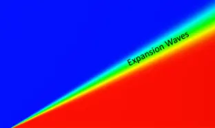
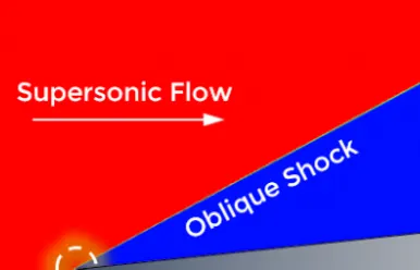
- Each line in the wave represents a line of constant properties. There are an infinite number of waves emanating from the corner and each wave will turn the flow a small amount, leading to a differentiating model.
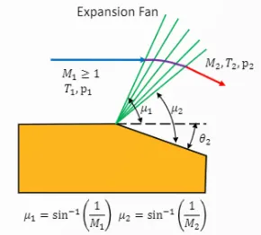

This is known as Prandtl Meyer Equation. This equation has to be integrated in order to achieve the final solution for the expansion wave.

The above expression is the final form after integration and is known as Prandtl Meyer Function.
When the upstream flow turns through an angle, the flow accelerates to a unique Mach number M2 which depends only on the fluid property  and Initial Mach Number M1.
Finally, the deflection angle can be expressed as ;

Geometry:
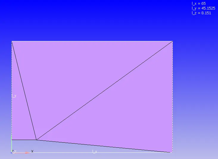
The geometry considered is about 65m in length along the x-direction and 45m along the y-direction. Along z-direction, the length can be ignored as the symmetric conditions can be applied and 2D sliced contours provide the same information as 3D at a much lesser computational effort.
Case setup:
Fluid: Air
Simulation type: Steady State
Turbulence Model: OFF
Solver: PISO-Density based
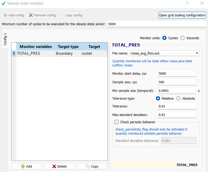
Steady State Monitor:
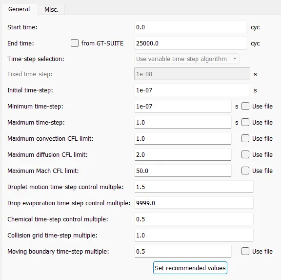
Simulation time parameters:
Boundary Conditions:
| Inlet | 101000.0 Pa, 678 m/s, 286K |
| outlet | Zero Normal Gradient |
| Top and Bottom faces | Wall |
| Front and Back faces | 2D symmetry |
Type of boundary condition for shock flow:
In compressible flows, the inlet velocity of the domain is generally known. Hence a constant value is given at the inlet(Dirichlet). However the outlet condition is not known priorly due to variations such as shocks which leads to gradient across the normal surface. This can be extrapolated from inlet condition and the basic properties of flow by defining the gradient to be zero.So, a neumann boundary condition is applied at the outlet.
Initial conditions:
Velocity = 678m/s, Pressure 50000 Pa, Temperature 300K
Grid Generation:
The grid is defined to be 0.8m along all 3 directions x,y, and z which provides around 44000 cells.
Adaptive mesh refinement:
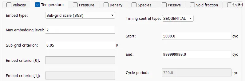
A temperature-based AMR is applied with a Sub-grid scale embedding level of 2 and a criterion is set to be 0.05 difference with respect to temperature curvature ( ). Here, in this case of expansion shock simulation, AMR can be applied to either pressure, velocity, or temperature as all 3 quantities experience a change proportionately.
AMR increases the cell count by the following relation,

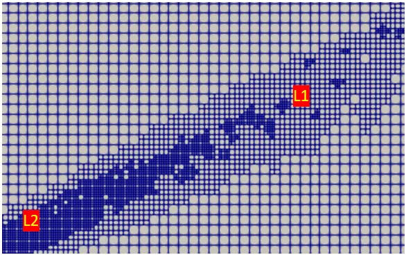
The above relation shows that as the embedding level is increased, the grid size is reduced which is evident in the below figure where the size of the grid at L2 is comparatively small than L1.
Results:
Case 1: Sub Grid Criterion = 0.05
Mesh: (Click here)
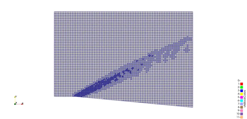
The above grid is generated with an SGS parameter of 0.05. The region at the middle with fine grids are a result of abrupt change in properties (here temperature, as SGS is applied to temperature curvature variation)
Pressure & Velocity Contours:
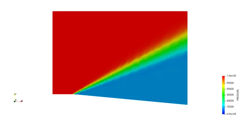
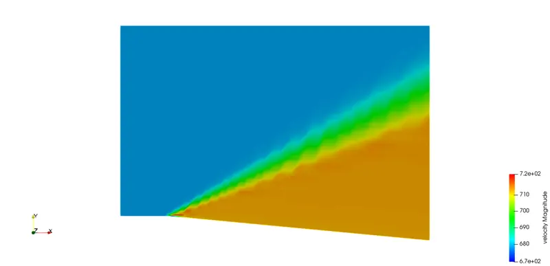
Fig. Pressure contour (Left), Velocity contour (Right)
The above contours show the variation of pressure and velocity. As the flow experiences a sudden expansion at a convex corner, properties such as pressure and velocity show abrupt change due to expansion fan formation. Development of pressure can be found here and development of velocity can be found here.
Case 2: Sub Grid Criterion = 0.01
Mesh: (Click here)
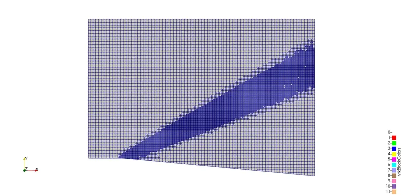
The above grid is generated with an SGS parameter of 0.01. The transition region of shock is well refined than the previous case of SGS 0.05. This leads to a more accurate value of flow properties.
Pressure & Velocity Contours:
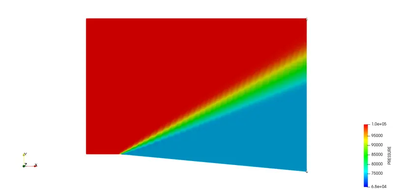
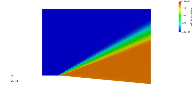
Fig. Pressure contour (Left), Velocity contour (Right)
The above contours of pressure and velocity are obtained for SGS 0.01. Development of pressure can be found here and development of velocity can be found here
Case 3: Sub Grid Criterion = 0.005
Mesh: (Click here)
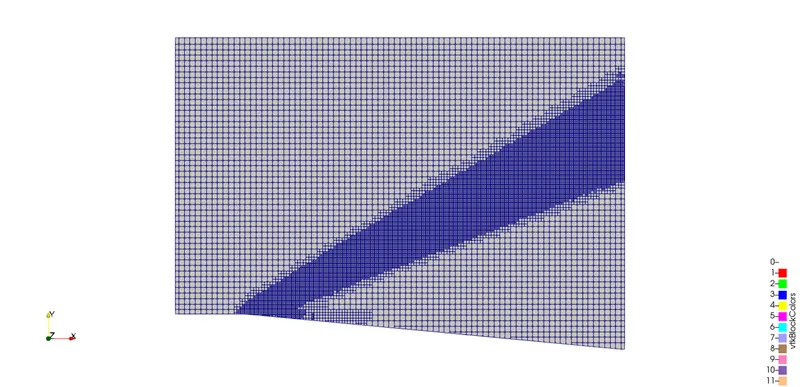
The above grid is generated with an SGS parameter of 0.005. The grid is refined with a 10x scale further which has produced a much finer mesh across the shock flow path and the region looks highly uniform.
Pressure & Velocity Contours:
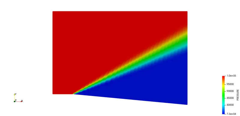
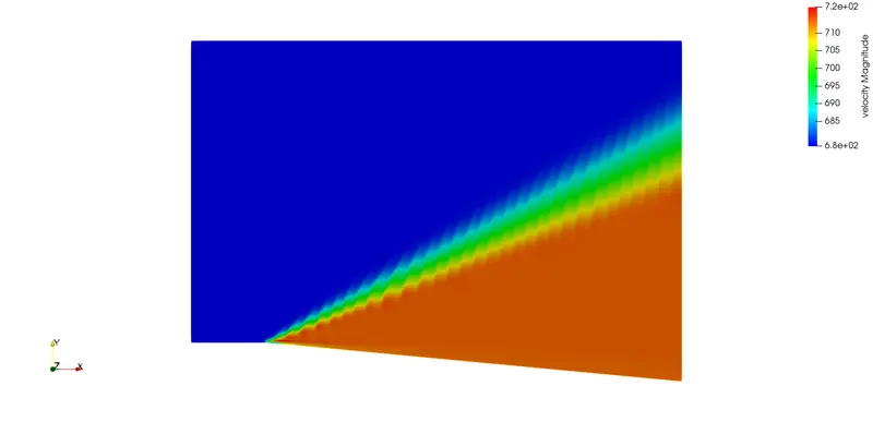
The above contours of pressure and velocity are obtained for SGS 0.005. Development of pressure can be found here and development of velocity can be found here.
Case 3: Sub Grid Criterion = 0.001
Mesh: (Click here)
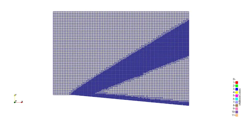
The above grid is generated with an SGS parameter of 0.001. The grid is refined in regions where there is no abrupt change of properties. This results in more computation without any yield of accuracy improvement. So an SGS of 0.005 is well sufficient if better accuracy is required.
Pressure & Velocity Contours:
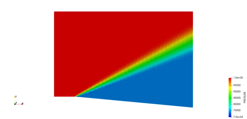
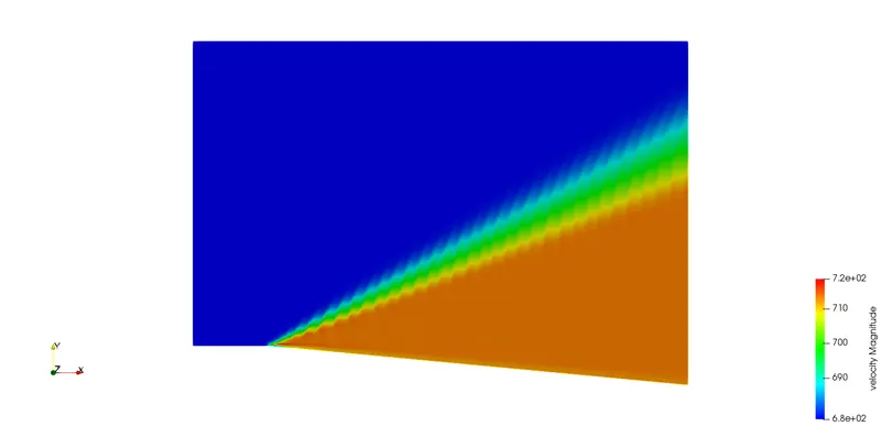
The above contours of pressure and velocity are obtained for SGS 0.001. Development of pressure can be found here and development of velocity can be found here.
Effect of SGS on Shock Location:
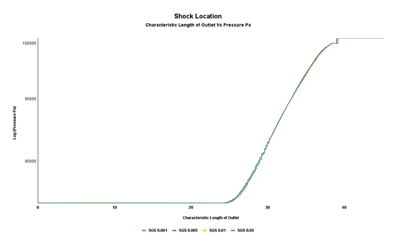
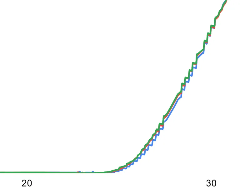
The above plot depicts the variation of Pressure across the outlet. The characteristic length of the outlet is around 50m of which the shock wave that emerged from the convex corner meets the outlet at around 25m. However, the plot below, which is a magnified view of variation between 25m and 30 m shows that there is a noticeable change in the deviation of shock location between the SGS parameters. The pressure variation is considered to be logarithmic for better visualization.
Effect of SGS Parameters on Cell count:
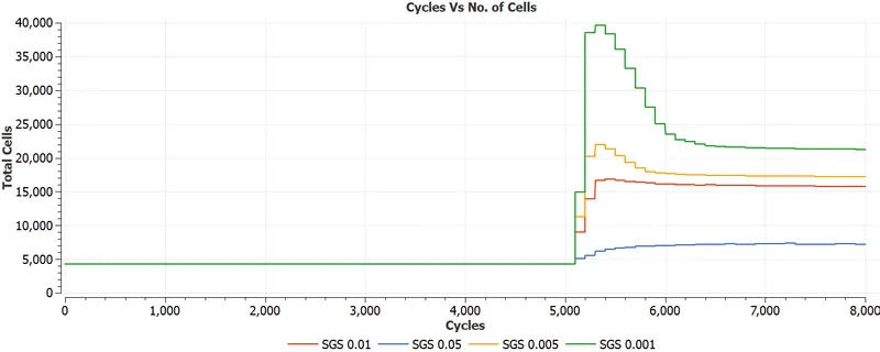
The above plot relates the variation between the number of cycles and total cell count in relation to the SGS parameter. It is very much obvious as the Subgrid scaling is decreased, cell count is increased leading to a more accurate solution.
Variation of Mach Number across the flow regime:
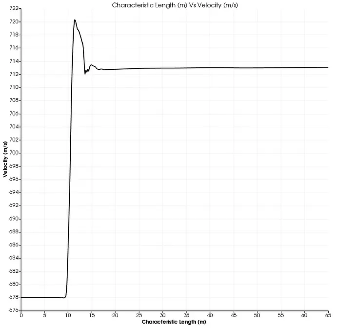
In the above plot, horizontal axis denotes the length of the region which reads to 65m. The vertical axis denotes the velocity across the length. It is evident that the Mach number is 1.97 at the initial state till the flow reaches around 8m. After 8m the flow accelerates with a Mach number of 2.1 as the flow meets a convex corner and then normalises to 2.07. The variation of velocity is due to the expansion wave formation after striking the convex corner.
Inferences:
- When a supersonic flow meets a convex corner, it forms an expansion fan leading to a spontaneous change of parameters such as velocity, pressure, and temperature.
- Properties such as Pressure and Temperature decreases downstream whereas Mach Number increases.
- As the Subgrid scaling parameter is decreased, the total cell count is increased.
- Due to an increase in cell count with a decrease of SGS, a more accurate shock location can be obtained.
References:
[2] https://en.wikipedia.org/wiki/Prandtl%E2%80%93Meyer_expansion_fan