Week - 5 - Modelling Spotwelds

Assignment 5

This assignment is dedicated to analyse and compare the behaviours of two distinct ways of modelling spot welds. First, we are going to model the spot welds with resort to beam elements and run a simulation. Afeter the results are obtained, the spot welds are going to be modified in order to be represented by 3D elements.

1. Weld definition

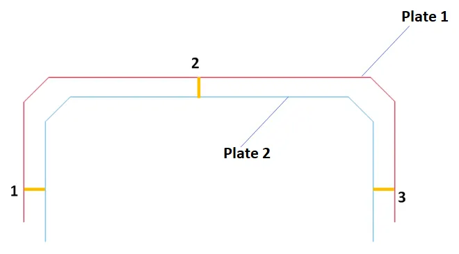
For reasons of simplicity, only 3 spot welds were created. The locations for the spot welds are the following:

2. Unit system

For reasons of convenience, the chose unit system is mm-ton-s.

3. Material definition

The material chose for both plates is steel (similar to assignment 4).

The properties of steel are:

Young's Modulus: E = 200 GPa = 200 000 MPa

Density: `\rho = 7800 {Kg }/m^3 = 7800 {1 \t\on }/(1000 mm)^3 = 7800 \times 10 ^{-9} \frac{\t\on}{mm^3} = 7.8 \times 10^{-12}\frac{\t\on}{mm^3}`

Poisson ratio: `\nu = 0.3`

The type of material to be defined is linear elastic (MAT_ELASTIC)

3. Shell section definition

In both plates, a thickness of 1.5 mm is used. The element formulation selected is Belytschko-Tsay.

In the Parts keyword, these sections were associated to both the plates.

4. Spot weld definition

To facilitate the spot weld element definition, the following section view was used:

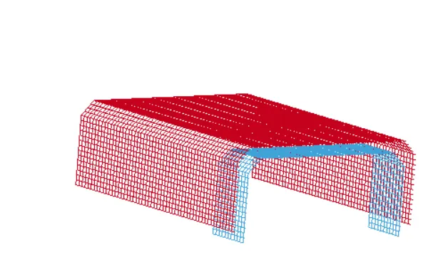
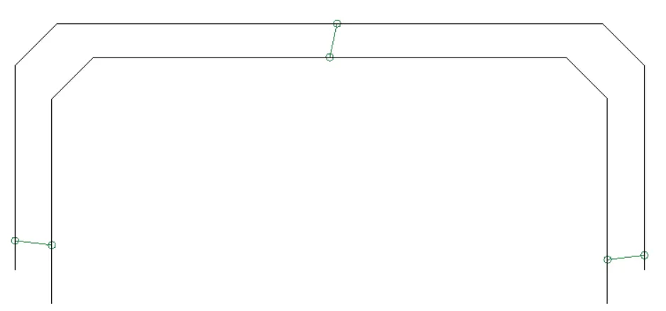
3 different beam elements were created in 3 different parts. Then, I moved all the elements to the same part by using the 'move or copy' menu.

The beam elements created are displayed in the next figure.

4.1. Spot weld material

To model the spot weld, MAT 100 was used. The mechanical properties used previously to define steel were also used to define this material.

As mentioned in the statement of the assignment, it is ideal that the welds fail at 50% of the total simulation time. So, it is clear that a time failure must be defined in the MAT 100 keyword. In one of the following sections, where the total simulation time is calculated, I will also calculate this failure time.

To avoid errors, the Yield Stress was set at 1% of the Young's Modulus, which is the default value assumed by the program.

4.1. Contacts for the welds

The beam elements connect 3 distinct nodes in Plate 1 to 3 distinct nodes in Plate 2.

In order to establish a contact that approximates the behaviour of an actual weld, the TIED_SHELL_EDGE_TO_SURFACE keyword was used.

In this keyword, the 6 nodes corresponding to the tips of the beam elements were put together in Node Set 1. Node Set 1 was then used as the slave set.

In the other hand, Plates 1 and 2 were out together in Part Set 1. This Part Set was defined as the Master Set of the contact.

5. Contact

A AUTOMATIC_SINGLE_SURFACE keyword was created to cover the plates coming into contact with each other due to sever deformation.

6. Boundary conditions

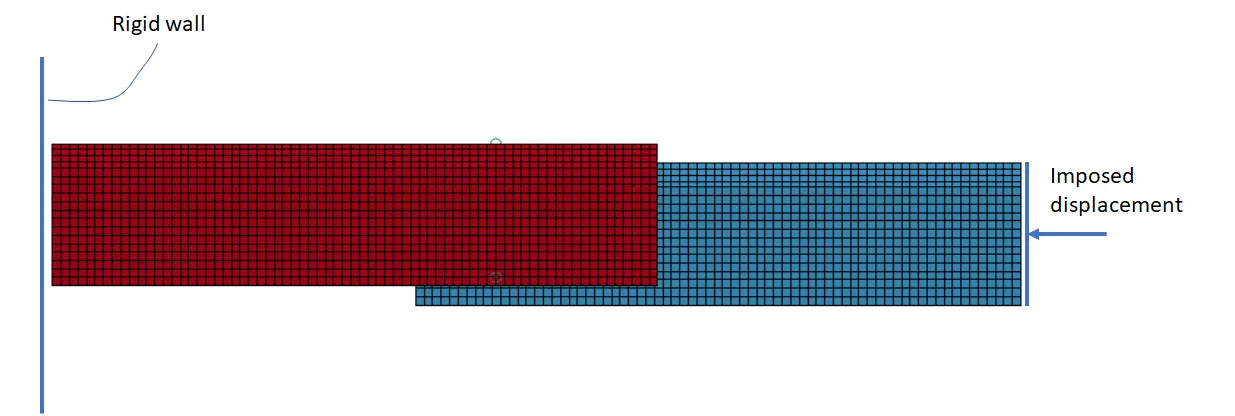
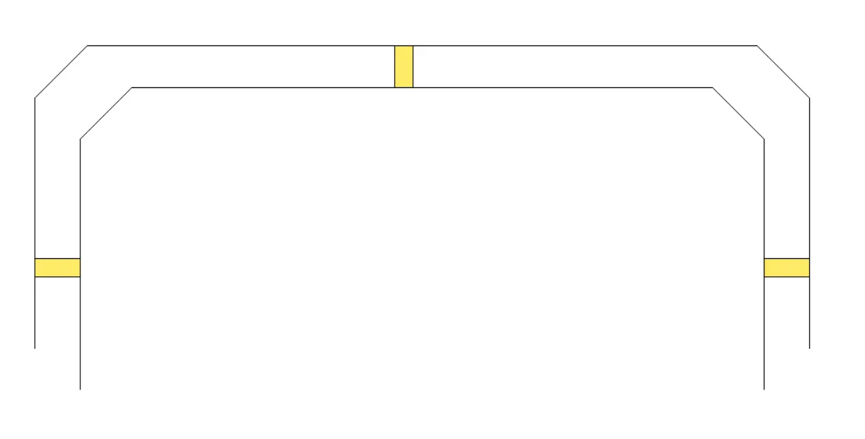
In this example, I will constraint the left-most edge of Plate 1 and impose a displacement of 50 mm in the opposite edge, as it can be seen in the following figure.

6.1. Imposed displacement

For this simulation, the right-most edge of the model is force to move along the x direction. This condiction involves an imposed displacement of 50 mm in a time span of 5 s (total simulation time).

Given a total simulation time of 5s, it can now be calculated that the failure time for the weld material must be 2.5s, as mentioned in section 4.1.

7. Rigid wall definition

The rigid wall was created so that it sits paralled to the left-most edge of the model, 1 mm to the left of it. The following figure shows the rigidwall that was defined.

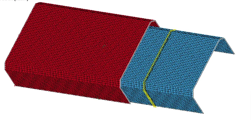
8. Cross section definition

The following cross section was defined to collect the cross sectional forces experienced during the crash.

9. Node result acquisition

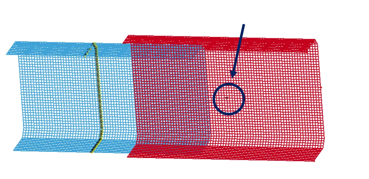
The node shown in the following figure was selected to extract the values for the acceleration in that particular node

10. Simulation controls

10.1. CONTROL_TERMINATION

This keyword must be defined in order to run the simulation. The simulation time was set to 5s

10.2. CONTROL_ENERGY

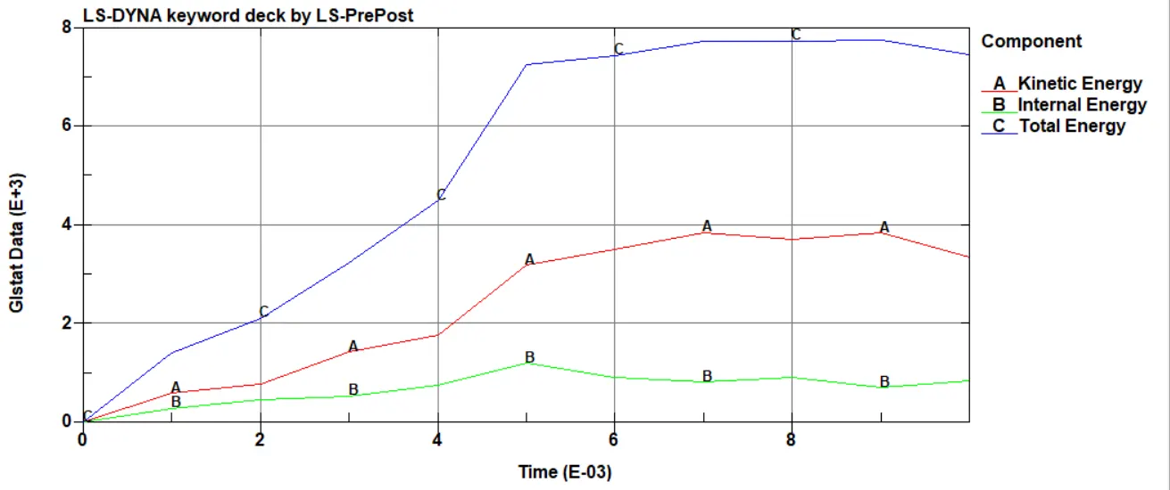
By defining this keyword and setting HGEN = 2, the hourglass energy can be computed and taken into account for the total energy calculations.

11. Outputs

The following keywords were activated:

- DATABASE_BINARY_D3PLOT - 3D plot extraction

- DATABASE_EXTENT_BINARY - Strain tensor calculation

- DATABASE_SECTION_SET - Cross Sectional forces

- HISTORY_NODE_SET - - kinematic data about the nodes

In the ASCII options, the following options were selected:

- GLSAT

- MATSUM

- NODOUT

- SECFORC

12. Results

12.1. Node accelerations

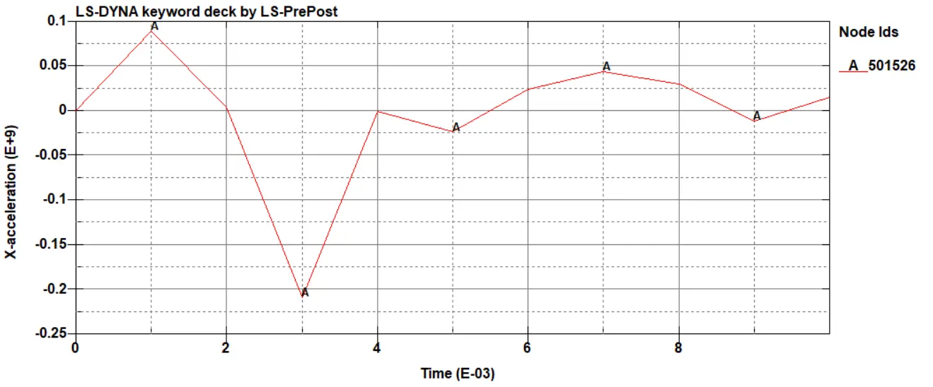
Recalling the node mentioned in section 9, the following x-accelerations were registered:

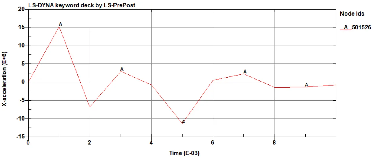
Since a constant velocity was imposed, it is normal that the acceleration of this node acquires an average value similar to zero troughout the simulation.

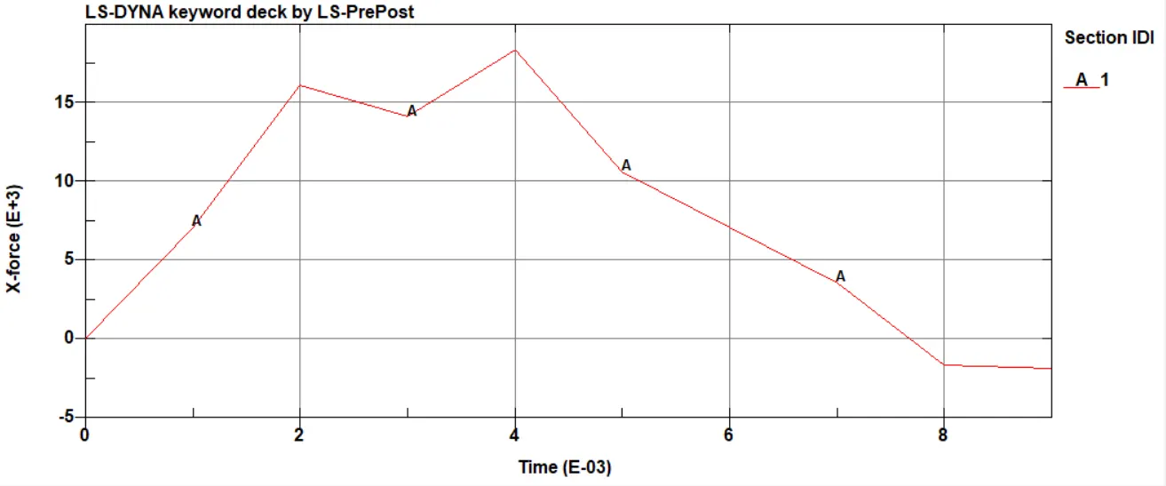
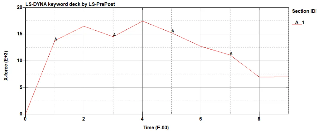
12.2. Cross-sectional forces

Recalling the node mentioned in section 9, the following x-accelerations were registered:

12.3. Model energies

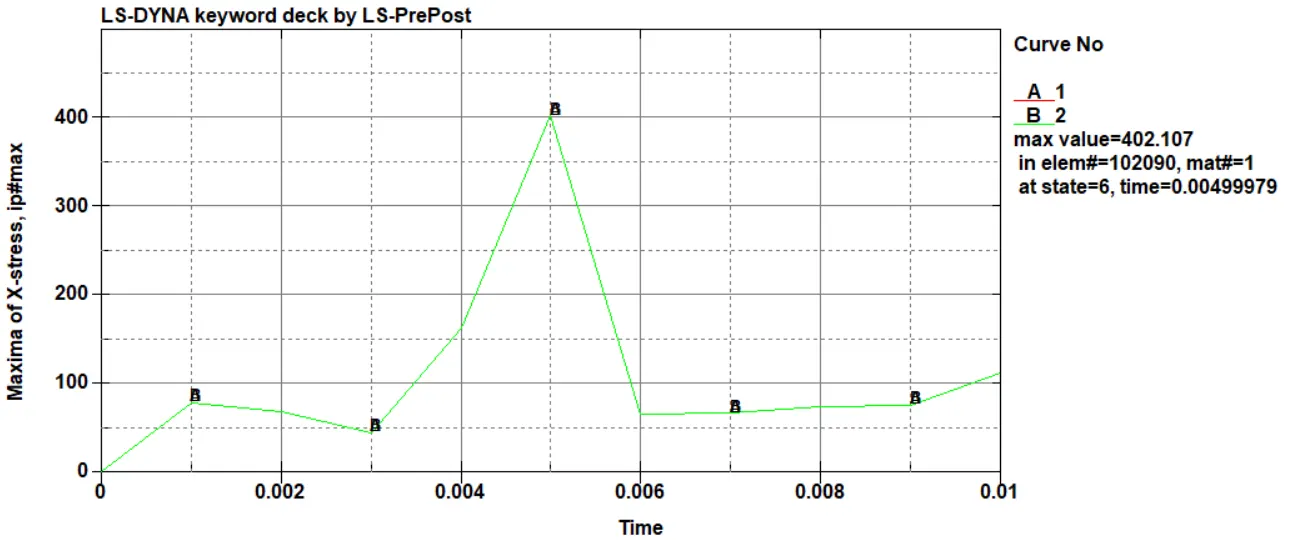
12.4. Maximum x-stress

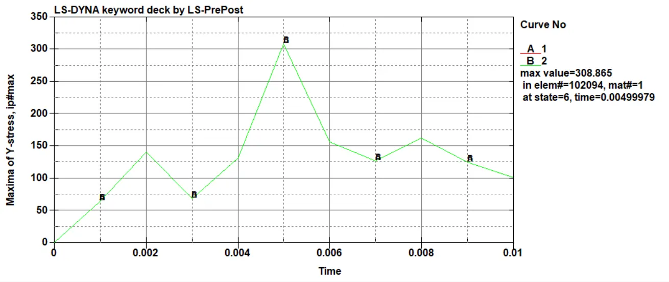
12.5. Maximum y-stress

12.6. Maximum z-stress

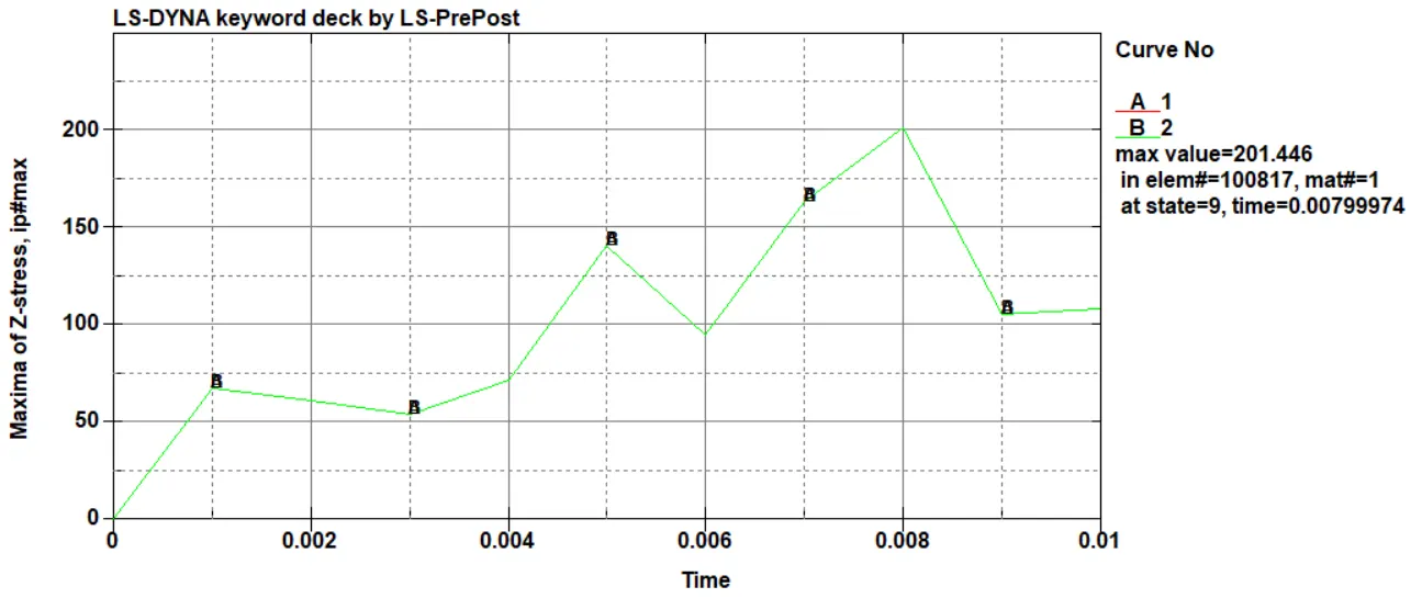
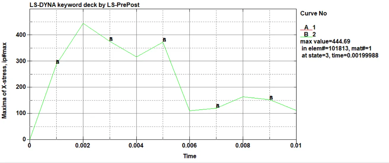
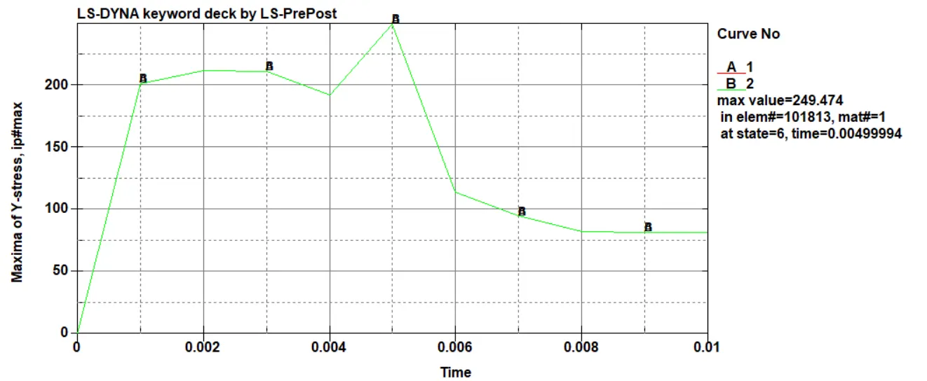
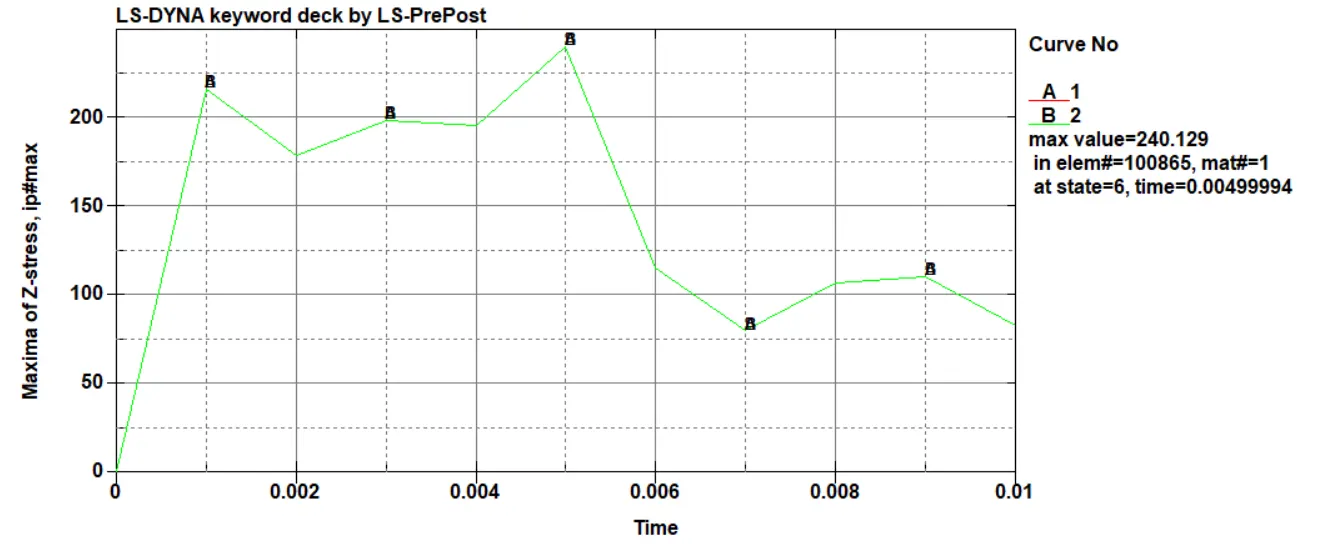
A peak of all stresses is seen close to when the spot weld elements fail, meaning that the fact that the spot weld elements fail allows stresses to be reduced from a particular time instead of keeping increasing.

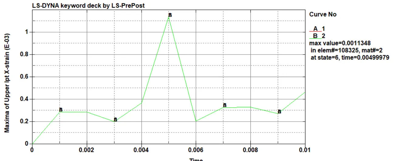
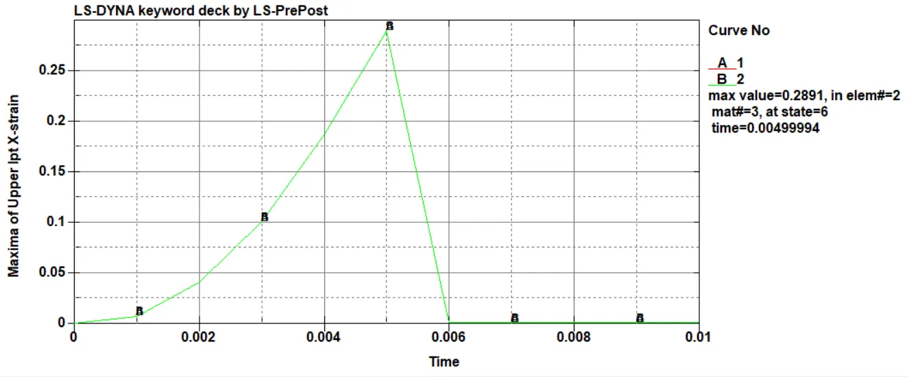
12.7. Maximum x-strain

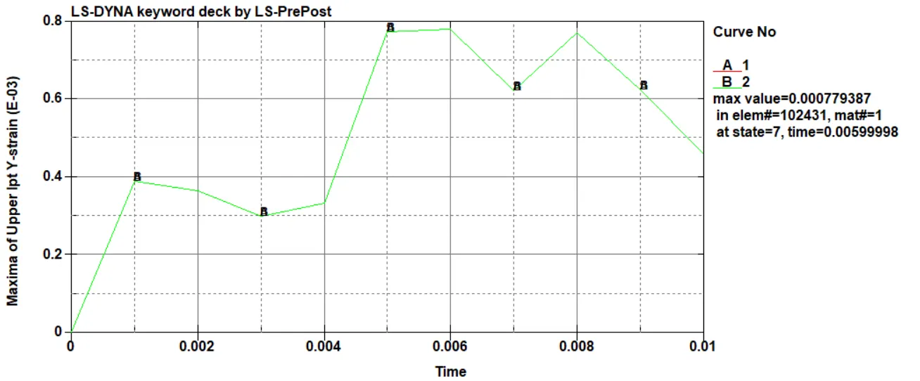
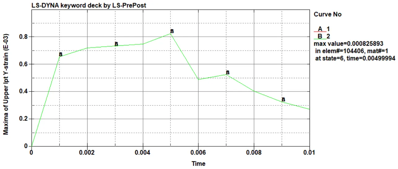
12.8. Maximum y-strain

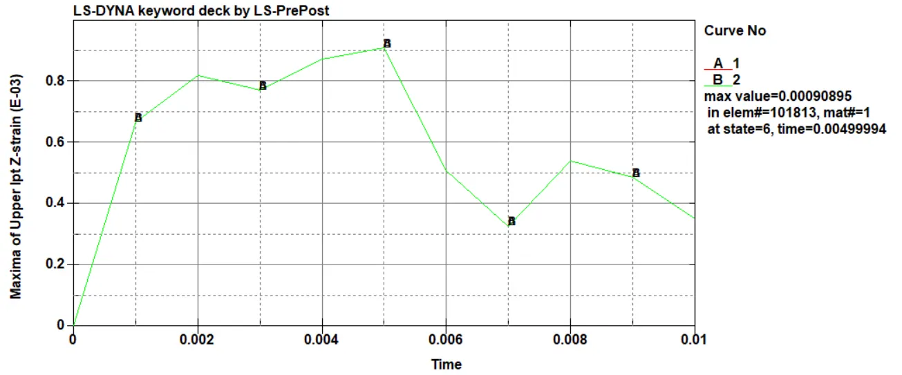
12.9. Maximum z-strain

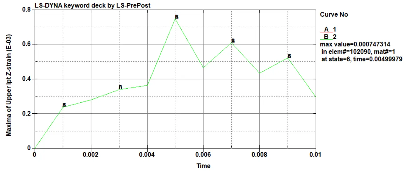
Similiarly to the case of stresses, there is also a moment half-way trough the simulation in which the strains reach a maximum value.

13. Spot welds modelled with solid elements

From now on, the model has been changed, and the 3 spot welds will now be modelled via 3 solid elements instead of 3 beam elements.

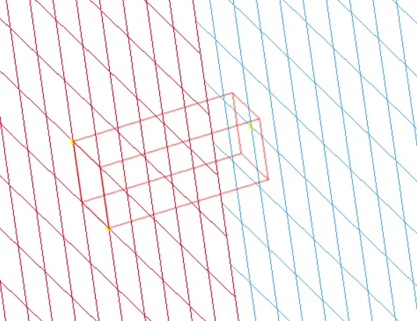
First, a box was created by defining two opposite base nodes in plate 1 and selecting a third node to define the height. The resuting geometry is shown in the following figure.

Then, this box was meshed by one solid element. The procedure was repeated for the other two elements

Another modification that was needed was the definition of a Solid section to be referenced in the part that represents the spot welds. The element formuation 1 was used.

A 'surface to surface' type of contact was created to establich connectivity between both parts. The elements of the plates that were in direct contact with the solid weld element were selected to the contact, as shown in the following figure.

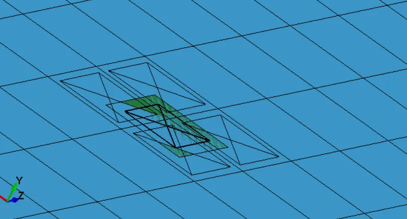
The following image shows the model ready for running the simulation.

14. Results - Solid spot weld elements

14.1. Node accelerations

14.2. Cross sectional forces

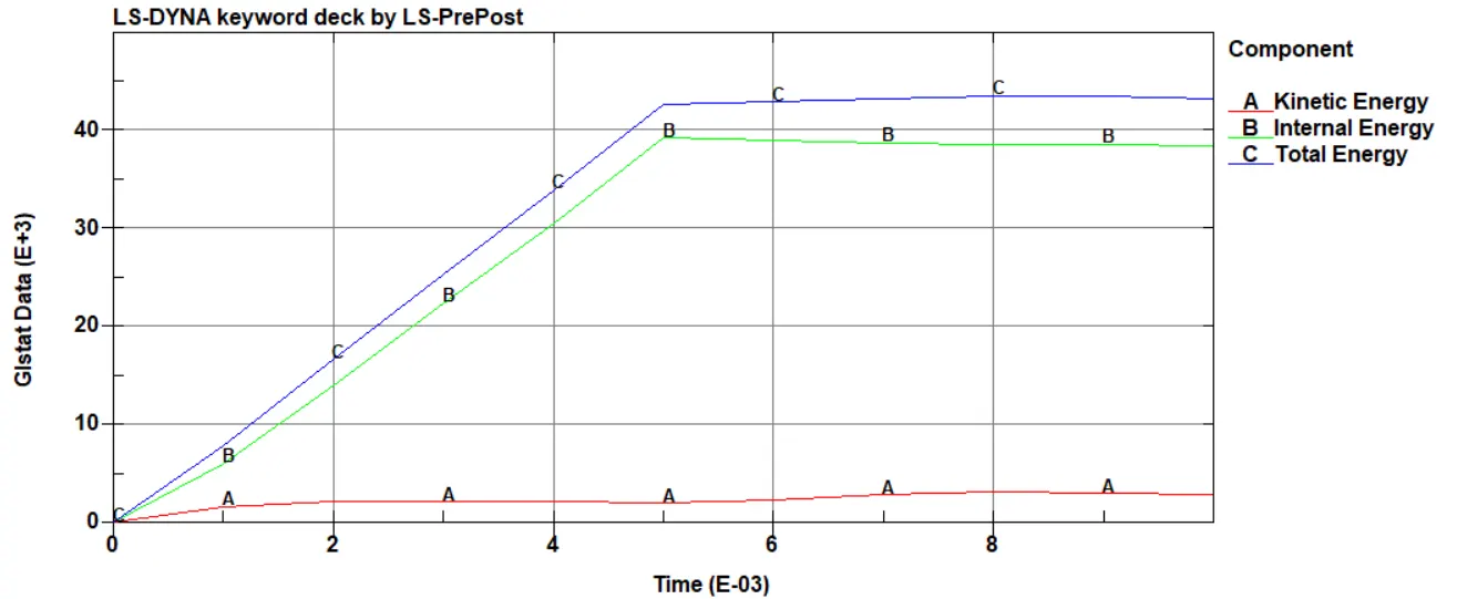
14.3. Model energies

14.4. Maximum x-stress

14.5. Maximum y-stress

14.6. Maximum z-stress

14.7. Maximum x-strain

14.8. Maximum y-strain

14.9. Maximum z-strain

15. Conclusions

• The plots for the maximum stresses and strains are almost coincident in both plates. This means that the maximum values are always observed in a connection point between them, which is one of the spot welds
• For both cases, the cross sectional force ends in a value close to zero. This is due to the deletion of the spot weld elements that cause a disconnection between the plates, preventing any force from being registred in the cross-section.
• The node acceleration has an average value of zero in both cases.
• Due to the larger dimensions of the spot welds, the total energy in the case of solid element spot welds is 5x bigger