Steady and Unsteady 2-D Heat Conduction (using GNU Octave)
2-D HEAT CONDUCTION - Steady & Transient State solutions
The idea is to simulate heat conduction phenomenon over a 2D planar geometry subjected to specified boundary condition for temperature, using numerical discretization and iterative solvers.
The solution is sought for both Steady and Unsteady/ Transient state of conduction. Also, three different iterative solvers are implemented for this computation- (i) Jacobi, (ii) Gauss-Seidel and (ii) Successive-Over-Relaxation (or SOR).
Visualizing the problem geometry:-
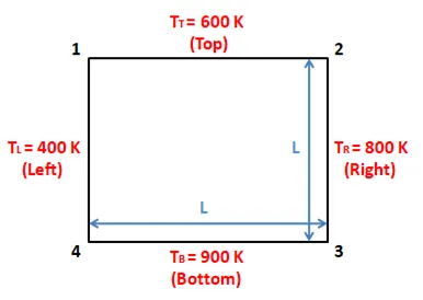
2D geometry is kept the same for both Steady and Transient State conduction. The peripheral temperatures for all four sides of the 2D plane are treated as the boundary conditions. For simplicity, the domain dimensions are taken as unit meter (i.e. 1 square-meter area). The temperature values of the four corners are taken as the average of the adjacent boundary temperatures.
The plane is dicretized into a mesh with equal nodes (12 nodes) in the horizontal (X) and the vertical (Y) direction. As the conduction equation consists of PDE terms that are of elliptical type, central differencing scheme for the space derivative terms to gather information from nodes on both X & Y axes aids in decretizing and computing the governing equation at each of the internal nodes.
STEADY STATE SOLUTION
The priliminary equation for Steady State conduction is expressed as follows:
`(del^2 T)/(del x^2) + (del^2 T)/(del y^2) = 0`
Upon dicretizing the above elliptical type PDEs using central differencing scheme, we get
`[ (T_(i+1,j) – 2T_(i,j) + T_(i-1,j))/(Delta x^2) ] + [ (T_(i,j-1) – 2T_(i,j) + T_(i,j+1))/(Delta y^2) ] = 0`
On simplifying further, we obtain the final expression for `T_(i,j)` as
`T_(i,j) = (1/k) [ ((T_(i+1,j) + T_(i-1,j))/(Delta x^2) ) + ( (T_(i,j-1) + T_(i,j+1))/(Delta y^2) ) ]` …… Eqn (1)
Where `k = (2(Delta x^2 + Delta y^2))/( Delta x^2 * Delta y^2)`
The equation can be further modified with the number of nodes in X & Y directions being the same, making `Delta x^2 = Delta y^2` (or dx = dy). The program code however, employs the general expression as the derived Eqn(1) in order to maintain variable versatility.
Program Code
To begin the computation, values of the internal nodes of the Temperature Field are assigned a guess value of 298 K. In order to facilitate convergence of the solution, a desired ‘tolerance’ for the final solution is set, which is compared with an ‘error’ term during each iteration. The iterations of this convergence loop continue until the ‘error’ falls within the tolerance limit, yielding the converged solution.
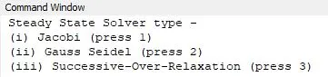
Three different iterative solvers are wriiten to solve the final expression of Steady State conduction. An input is taken from the user for the choice of solver, accoridng to which the corresponding code block is executed. The solver also keeps track of the number of iterations and the evaluation time taken to reach solution convergence. Acquired results are then depicted as Temperature Contours with appropriate scaling.
As time derivative term is equated to zero in case of steady state simulation, iterations based on time-steps gets omitted due to absence of any coupled linear expressions and thus, the solution type can be essentially thought of as Explicit Intergration
The program code including explanatory comments is as follows:
% STEADY STATE 2D HEAT CONDUCTION CODE
clear all;
close all;
clc;

L = 1;           % Domain Area as 1 square-meter
nx=12; ny=12;    % Grid points in X and Y direction resp.
% Creating the Mesh and determing the grid spacings in X and Y directions
x=linspace(0,L,nx); dx=x(2)-x(1);
y=linspace(0,L,ny); dy=y(2)-y(1);
y0=fliplr(y);   % Reversing/Flipping Y-axis to aptly use in plotting

% Temperture Boundary Conditions
T = ones(nx,ny)*298 ; % Initial Guess Value for the Temperture Field
% Boundary Temperature Values
T(2:nx-1,1) = 400;   % Left
T(2:nx-1,ny) = 800;  % Right
T(1,2:ny-1) = 600;   % Top
T(nx,2:ny-1) = 900;  % Bottom
% Corner Temperature Values (as average of boundary values)
T(1,1) = (T(2,1)+T(1,2))/2;
T(1,end) = (T(1,2)+T(2,ny))/2;
T(end,1) = (T(nx-1,1)+T(nx,2))/2;
T(end,end) = (T(nx-1,ny)+T(nx,ny-1))/2;

error = 100;       % Initializing error variable
tolerance = 1e-4;  % Defining requisite tolerance for solution convergence
t_old = T;         % Variable to store values from previous iteration
iteration_count=0; % Variable to count completed interations upto convergence
k = (2*((dx^2)+(dy^2)))/((dx^2)*(dy^2));

% Taking user input for choice of Iterative Solver
iterative_solver= input(" Steady State Solver type - n (i) Jacobi (press 1) n (ii) Gauss Seidel (press 2) n (iii) Successive-Over-Relaxation (press 3) n");

% Computing the various solutions based on the user input
if iterative_solver==1  % JACOBI METHOD
  tic;     % Start timer
  % CONVERGENCE LOOP
    while (error>tolerance)
      iteration_count=iteration_count+1; % Increment conunter for each iteration
         % SPACE LOOP to solve all 2D grid points
         for i = 2:nx-1
              for j = 2:ny-1
                 % Splitting the final expression for fool-proofing
                 A = (t_old(i-1,j)+t_old(i+1,j))/(dx^2);
                 B = (t_old(i,j-1)+t_old(i,j+1))/(dy^2);
                 T(i,j) = (1/k)*(A+B);
              endfor
         endfor
      error = max(max(abs(t_old-T))); % Determining maximum error value
      t_old = T;                      % Updating old values for next iteration

   endwhile
   t_eval = toc;  % Stop timer and store computation time

elseif iterative_solver==2  % GAUSS-SEIDEL METHOD
    tic; % Start timer
    % CONVERGENCE LOOP
    while (error>tolerance)
      iteration_count=iteration_count+1; % Increment conunter for each iteration
         % SPACE LOOP to solve all 2D grid points
         for i = 2:nx-1
              for j = 2:ny-1
                  % Splitting the final expression for fool-proofing
                  A = (T(i-1,j)+t_old(i+1,j))/(dx^2);
                  B = (T(i,j-1)+t_old(i,j+1))/(dy^2);
                  T(i,j) = (1/k)*(A+B);
              endfor
         endfor
      error = max(max(abs(t_old-T))); % Determining maximum error value
      t_old = T;                     % Updating old values for next iteration

   endwhile
   t_eval = toc;        % Stop timer and store computation time

elseif iterative_solver==3  % SOR METHOD
   omega = 1.2;   % Relaxation Factor
   tic;           % Start timer
   % CONVERGENCE LOOP
     while (error>tolerance)
       iteration_count=iteration_count+1; % Increment conunter for each iteration
         % SPACE LOOP to solve all 2D grid points
         for i = 2:nx-1
              for j = 2:ny-1
                  % Splitting the final expression for fool-proofing
                  A = (T(i-1,j)+t_old(i+1,j))/(dx^2);
                  B = (T(i,j-1)+t_old(i,j+1))/(dy^2);
                  T(i,j)= ((1-omega)*t_old(i,j)) + ((omega/k)*(A+B));
              endfor
         endfor
      error = max(max(abs(t_old-T))); % Determining maximum error value
      t_old = T;                      % Updating old values for next iteration

   endwhile
   t_eval = toc;    % Stop timer and store computation time

endif

 % PLOTTING THE TEMPERATURE CONTOUR
figure (1)
contourf(x,y0,T);
[C,H] = contourf(x,y0,T);
colorbar;
colormap(jet);
clabel(C,H);
xlabel('X-direction'); ylabel('Y-direcction');
title_text=sprintf('n2D HEAT CONDUCTION - STEADY STATE SOLUTION n Iteration Count = %d ; Computation Time = %d sec', iteration_count,t_eval);
title(title_text);
Input via Command Window:
Results
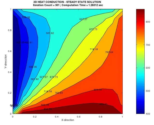
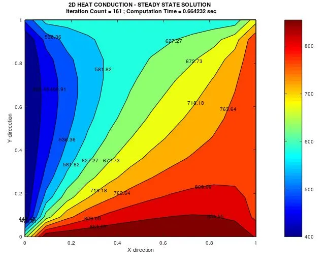
The following are the temperature contours plotted for each iterative solver methods:
(I) JACOBI METHOD
(II) GAUSS-SEIDEL METHOD
(III) SUCCESSIVE-OVER-RELAXATION (or SOR) METHOD
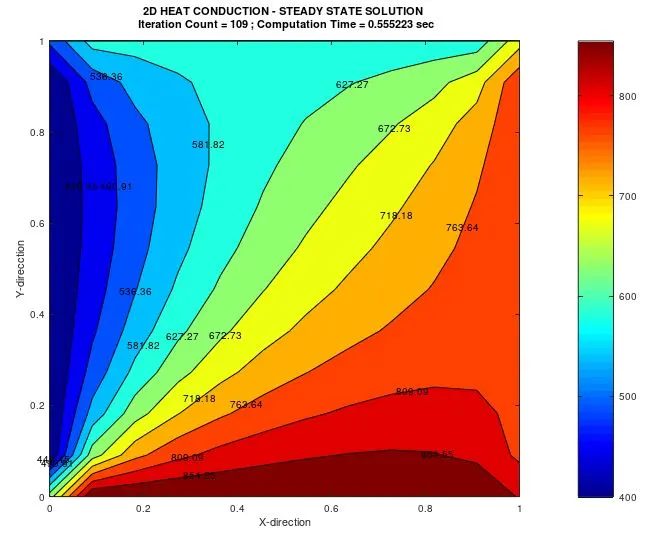
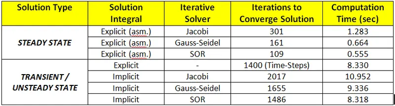
A glipse of performances of the iterative solvers can be observed from the number of iterations taken by the solver to reach solution convergence and proportionally, the time taken to do so. Jacobi method takes the highest time for the computation and runs 301 iterations whereas SOR attains convergence in 109 iterations thereby taking less time.
TRANSIENT (UNSTEADY) STATE SOLUTION
In case of transient state, the equation is expressed as-
`(del T)/(del t) = alpha [(del^2 T)/(del x^2) + (del^2 T)/(del y^2) ]`
As the equation consists of a time derivative term, the solution can be sought using both Explicit and Implicit Integration. Thus, a for-loop running sufficent number of time steps until the solution tends to steady state has to additionally included in the code block.
(i) EXPLICIT
The transient state equation is discretized as follows:
`(T_(i,j)^(n+1) – T_(i,j)^n)/(Delta t) = alpha [(T_(i+1,j) – 2T_(i,j) + T_(i-1,j))/(Delta x^2) + (T_(i,j-1) – 2T_(i,j) + T_(i,j+1))/(Delta y^2) ]^n`
Where `alpha =` Thermal Diffusivity
Upon simplification, we obtain the final expression as:
`T_(i,j)^(n+1) = T_(i,j)^n + k_1 (T_(i+1,j) – 2T_(i,j) + T_(i-1,j))^n + k_2(T_(i,j-1) – 2T_(i,j) + T_(i,j+1))^n` …..... Eqn (2)
Where `k_1 = (alpha Delta t)/(Delta x^2)` and `k_2 = (alpha Delta t)/(Delta y^2)` ; which are referred as CFL numbers, used for stabilty analysis of the solution.
Since the right-hand side of the equation (older time-step values) is readily solvable duirng each iteration to solve for the newer time-step, iterative solvers are not required here. A convergence may be used within the for-loop for time-step counting if desired, although the solution is expected to converge even by iterating with enough number of time-steps.
(ii) IMPLICIT
For implicit integration, Eqn (2) can be utilized by changing the time-step at which the right-hand side values are taken.
`T_(i,j)^(n+1) = T_(i,j)^n + k_1 (T_(i+1,j) – 2T_(i,j) + T_(i-1,j))^(n+1) + k_2(T_(i,j-1) – 2T_(i,j) + T_(i,j+1))^(n+1)`
Where again `k_1 = (alpha Delta t)/(Delta x^2)` and `k_2 = (alpha Delta t)/(Delta y^2)` [CFL numbers]
The equation can be further manipulated to obtain the final expression as:
`T_(i,j)^(n+1) = [ T_(i,j)^n + k_1 (T_(i+1,j) + T_(i-1,j))^(n+1) + k_2(T_(i,j-1) + T_(i,j+1))^(n+1) ]/((1+2k_1+2k_2))` ………. Eqn (3)
To compute this expression, all the three iterative solvers are employed i.e. Jacobi, Gauss-Siedel and SOR. Unlike explicit one, the code block for these solvers also consist of a convergence loop similar to as used in the steady state solution code.
However, it is crucial to note the loop within which the Temperature matrices update iteratively. The set of old values to be used for solution convergence have to be updated inside the convergence loop, while the temperature values from a preceeding time-step have to be updated outside the convergence loop (i.e. within the for-loop of time-steps).
Program Code
The initial code lines are similar to the program code for steady state, inclusive of mesh creation, defining boundary conditions, requisite variable assignment and user input is taken for the choice of solution integral – Explicit or Implicit.
Since explicit integral does not include any iterative solvers, the choice directly renders a problem solution. But, as different iterative solvers are employed under Implicit integral, user input is taken again as a sub-choice for the solver. This is implemented as nested if-else command within the program code, that executes the appropriate code block cooresponding to the choice of user to compute the solution.
General expressions as given by Eqn (2) & (3) are used instead of further reducing it using dx = dy, to retain the versatility of the program code. The number of iterations to converge and time taken to compute the same are also calculated to compare the three solvers. Final results are then rendered as suitable Temperature Contours.
The program code including explanatory comments is as follows:
clear all;
close all;
clc;

L = 1;                         % Domain Area as 1 square-meter
nx=12; ny=12;                  % Grid points in X and Y direction resp.
% Creating the Mesh and determing the grid spacings in X and Y directions
x=linspace(0,L,nx); dx=x(2)-x(1);
y=linspace(0,L,ny); dy=y(2)-y(1);
y0 = fliplr(y);  % Reversing/Flipping Y-axis to aptly use in plotting
% Defining the Number of Time-Steps
t_end = 700; dt=0.5;
t_n = t_end/dt;

% Temperture Boundary Conditions
T = ones(nx,ny)*298 ; % Initial Guess Value for the Temperture Field
% Boundary Temperature Values
T(2:nx-1,1) = 400;   % Left
T(2:nx-1,ny) = 800;  % Right
T(1,2:ny-1) = 600;   % Top
T(nx,2:ny-1) = 900;  % Bottom
% Corner Temperature Values (as average of boundary values)
T(1,1) = (T(2,1)+T(1,2))/2;
T(1,end) = (T(1,2)+T(2,ny))/2;
T(end,1) = (T(nx-1,1)+T(nx,2))/2;
T(end,end) = (T(nx-1,ny)+T(nx,ny-1))/2;

error = 100;       % Initializing error variable
tolerance = 1e-4;  % Defining requisite tolerance for solution convergence
t_old = T;         % Variable to store values from previous iteration
Prev_T = T;        % Variable to store values from previous Time-Step
iteration_count=0; % Variable to count completed interations upto convergence

% Taking user input for choice of Solution Integral
printf("TRANSIENT 2D HEAT CONDUCTION n");
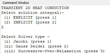
ans = input("Select solution integral:- n (1) EXPLICIT [press 1] n (2) IMPLICIT [press 2] n");

% Computing the various solutions based on the user input
if ans ==1    % EXPLICIT
   alpha=1e-3; % Thermal diffusivity
   k1=(alpha*dt)/(dx^2); k2=(alpha*dt)/(dy^2); % Calculating CFL values
   tic;    % Start timer
   % For-loop to count the number of Time-Steps
   for nt=1:t_n

         % SPACE LOOP to solve all 2D grid points
          for i=2:nx-1
             for j=2:ny-1
               % Splitting the final expression for fool-proofing
               A = k1*(t_old(i-1,j)-2*t_old(i,j)+t_old(i+1,j));
               B = k2*(t_old(i,j-1)-2*t_old(i,j)+t_old(i,j+1));
               T(i,j) = t_old(i,j) + A + B;
             endfor
          endfor
        error=max(max(abs(t_old-T)));  % Determining maximum error value
        t_old=T;                       % Updating old values for next iteration
        iteration_count=iteration_count+1; % Increment conunter for each iteration

     endfor
     t_eval = toc;  % Stop timer and store computation time

   % PLOTTING THE TEMPERATURE CONTOUR - EXPLICIT
    figure (1)
    contourf(x,y0,T);
    [C,H] = contourf(x,y0,T);
    colorbar;
    colormap(jet);
    clabel(C,H);
    xlabel('X-direction'); ylabel('Y-direcction');
    itle_text=sprintf('2D HEAT CONDUCTION - TRANSIENT STATE SOLUTION [EXPLICIT] n Iteration Count = %d ; Computation Time = %d ', iteration_count,t_eval);
    title(title_text);

elseif ans==2   % IMPLICIT
   % Taking user input for choice of Iterative Solver
   iterative_solver = input("nSelect Solver type - n (i) Jacobi (press 1) n (ii) Gauss Seidel (press 2) n (iii) Successive-Over-Relaxation (press 3) n");

   alpha=1.3;                                   % Thermal diffusivity
   k1=(alpha*dt)/(dx^2); k2=(alpha*dt)/(dy^2);  % Calculating CFL values
   denom = 1+2*k1+2*k2;

   if iterative_solver==1  % JACOBI METHOD
     tic; % Start timer
     % For-loop to count the number of Time-Steps
     for nt=1:t_n
       error=100; % Re-initializing error term for each time-step loop
       % CONVERGENCE LOOP
         while (error>tolerance)
          iteration_count=iteration_count+1; % Increment conunter for each iteration
          % SPACE LOOP to solve all 2D grid points
              for i = 2:nx-1
                  for j = 2:ny-1
                    % Splitting the final expression for fool-proofing
                    A = k1*(t_old(i-1,j)+t_old(i+1,j));
                    B = k2*(t_old(i,j-1)+t_old(i,j+1));
                    T(i,j)= (Prev_T(i,j)+ A + B)/denom;
                 endfor
              endfor
           error = max(max(abs(t_old-T)));  % Determining maximum error value
           t_old = T;                       % Updating old values for next iteration
         endwhile
         Prev_T = T;                        % Updating old values for next Time-Step
       endfor
       t_eval = toc;  % Stop timer and store computation time

    elseif iterative_solver==2  % GAUSS-SEIDEL METHOD
    tic; % Start timer
    % For-loop to count the number of Time-Steps
    for nt=1:t_n
     error=100; % Re-initializing error term for each time-step loop
     % CONVERGENCE LOOP
       while (error>tolerance)
          iteration_count=iteration_count+1; % Increment conunter for each iteration
          % SPACE LOOP to solve all 2D grid points
             for i = 2:nx-1
                for j = 2:ny-1
                   % Splitting the final expression for fool-proofing
                    A = k1*(T(i-1,j)+t_old(i+1,j));
                    B = k2*(T(i,j-1)+t_old(i,j+1));
                    T(i,j)= (Prev_T(i,j)+ A + B)/denom;
                endfor
            endfor
      error = max(max(abs(t_old-T)));  % Determining maximum error value
      t_old = T;                       % Updating old values for next iteration

    endwhile
   Prev_T = T;                        % Updating old values for next Time-Step
  endfor
  t_eval = toc;  % Stop timer and store computation time

elseif iterative_solver==3 % SUCCESSIVE-OVER-RELAXATION METHOD
   omega = 1.2;  % Relaxation Factor
   tic;          % Start timer
   % For-loop to count the number of Time-Steps
    for nt=1:t_n
    error=100; % Re-initializing error term for each time-step loop
    % CONVERGENCE LOOP
     while (error>tolerance)
       iteration_count=iteration_count+1;  % Increment conunter for each iteration
       % SPACE LOOP to solve all 2D grid points
         for i = 2:nx-1
              for j = 2:ny-1
                 % Splitting the final expression for fool-proofing
                  A = k1*(T(i-1,j)+t_old(i+1,j));
                  B = k2*(T(i,j-1)+t_old(i,j+1));
                  T(i,j)= ((1-omega)*t_old(i,j)) + (omega*(Prev_T(i,j)+ A + B))/denom;
              endfor
         endfor
      error = max(max(abs(t_old-T)));  % Determining maximum error value
      t_old = T;                       % Updating old values for next iteration

     endwhile
     Prev_T = T;                      % Updating old values for next Time-Step
   endfor
   t_eval = toc;  % Stop timer and store computation time

endif

% PLOTTING THE TEMPERATURE CONTOUR - IMPLICIT
figure (1)
contourf(x,y0,T);
[C,H] = contourf(x,y0,T);
colorbar;
colormap(jet);
clabel(C,H);
xlabel('X-direction'); ylabel('Y-direcction');
title_text=sprintf('2D HEAT CONDUCTION - TRANSIENT STATE SOLUTION [IMPLICIT]n Iteration Count = %d ; Computation Time = %d ', iteration_count,t_eval);
title(title_text);


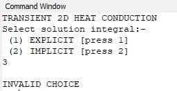
else
  printf("nINVALID CHOICEn");
endif
Input via Command Window:
Results
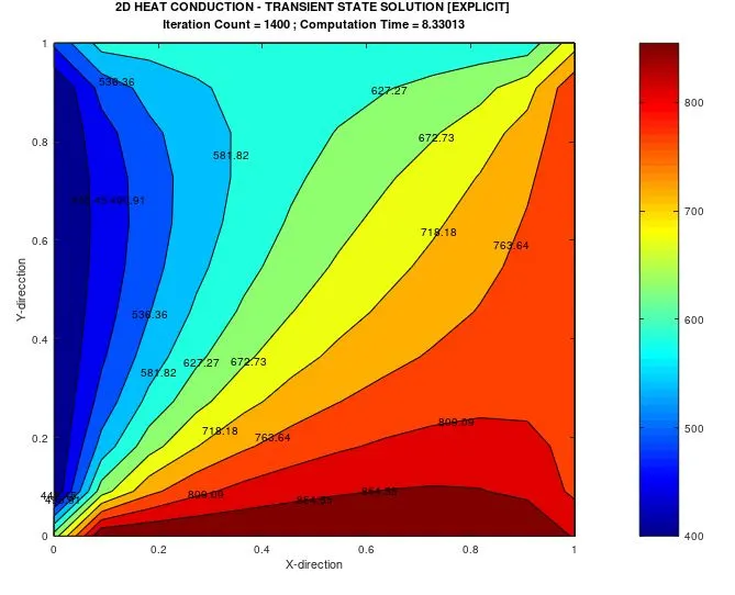
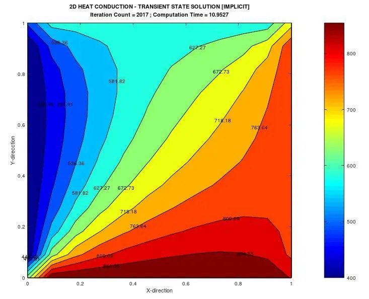
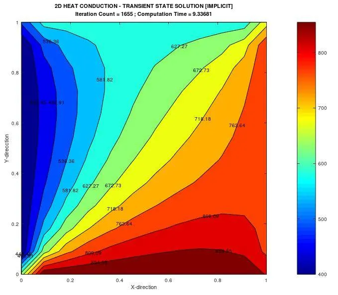
The temperature contours for each of the user choices are as follows:
(I) EXPLICIT
(II) IMPLICIT : JACOBI
(III) IMPLICIT : GAUSS-SEIDEL
(IV) IMPLICIT : SUCCESSIVE-OVER-RELAXATION (or SOR)
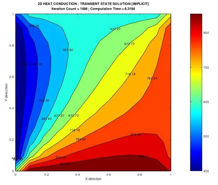
As evident from the computation time taken, all the implicit integrals take longer time compared to the explicit integrals.
Similar to the observation in the Steady State simulation, the SOR method takes lesser time to solve running 1486 iterations for convergence. On the other hand, Jacobi method takes 2017 iterations to reach convergence taking a comparatively longer computation time.
A summary table encompassing the recorded performance parameters is given below.