Week 5 - Literature review: ODE Stability

ODE STABILITY

Objective: In this challenge, literature review of ODE stability and how stability of the ODEs and the approches to solve the ODEs effect the solution result.

What is ODE ?

An ordinary differential equation (ODE) is a differential equation containing one or more functions of one independent variable and the derivatives of those functions. A differential equation is an equation that contains a function with one or more derivatives. But in the case ODE, the word ordinary is used for derivative of the functions for the single independent variable.

Stability, in mathematics, is a condition in which a slight disturbance in a system does not produce too disrupting an effect on that system. In terms of the solution of a differential equation, a function f(x) is said to be stable if any other solution of the equation that starts out sufficiently close to it when x = 0 remains close to it for succeeding values of x. If the difference between the solutions approaches zero as x increases, the solution is called asymptotically stable. If a solution does not have either of these properties, it is called unstable.

There are two type of approches namely Explicit method and implicit method. An explicit solution results from a method that is independent of other values (for the same level), a single equation is used to evaluate new variables for a single time step. An implicit solution contains information obtained from solving simultaneous equations for previous and current time step. This is computationally more demanding but allows for larger time steps and better stability.

'''
Python program to solve an ODE using both implicit(im) and explicit(em) methods.

comparing results with each other as well as with analytical solution.
'''
import matplotlib.pyplot as plt 
import numpy as np
import math

t_tot = 0.1 # total time the solution needs to be calculated.
dt = 1e-3 #timescale size
 
def em(t_tot,dt):

	t = np.arange(0,t_tot,dt)
	y = np.zeros(len(t))

	for i in range(1,len(t)):
		y[i] = y[i-1] + dt*(-1000*y[i-1] - np.exp(-t[i-1]))
	
	return [t,y]

def im(t_tot,dt):

	t = np.arange(0,t_tot,dt)
	y = np.zeros(len(t))

	for i in range(1,len(t)):
		y[i] = ( y[i-1]-dt*np.exp(-t[i-1]) )/(1+1000*dt)
	
	return [t,y]

def an(t_tot,dt):

	t = np.arange(0,t_tot,dt)
	y = np.zeros(len(t))

	for i in range(1,len(t)):
		y[i] = np.exp(-1000*t[i])*(1-np.exp(999*t[i]))/999
	
	return [t,y]


t,em = em(t_tot,dt) # assigning t and y values to t, em.
t,im = im(t_tot,dt)
t,an = an(t_tot,dt)
plt.plot(t,em,color='red')
plt.plot(t,im,color='blue')
plt.plot(t,an,color='green')
plt.legend(['Explicit','Implicit','Analytical'])
plt.title('Timestep size:'+ str(dt))	
plt.show()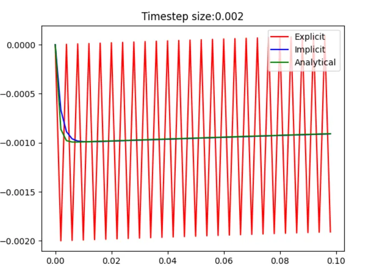

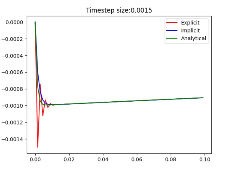
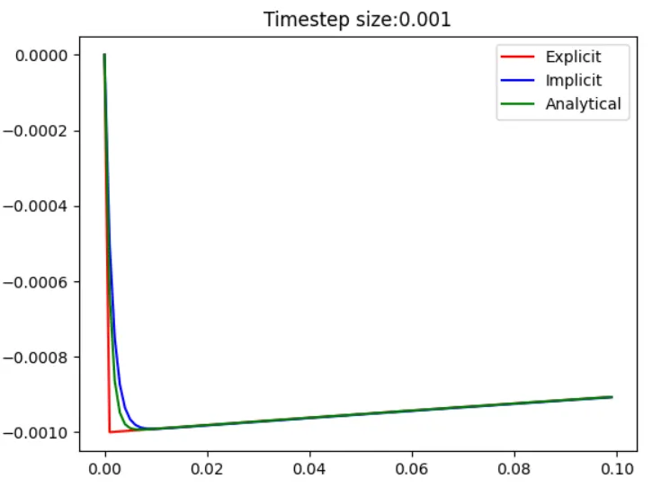
From the above graphs, it can observed that as the timestep size increased explicit method started diverging which means the solution became unstable whereas implicit method remained stable.

How does stability affect engineering simulations?

Stability plays a key role in getting the right values for the variables of the solution. Purpose of the numerical simulation is to optimize, understand the problem and find the prefect solution. when the solution is unstable we get unrelable values which are not desirable.

Can stability condition be derived for all types of problems ?

Stability condition can be derived for all types of ODEs. However the stability condition depends on type of ODE and the type of the solver. even if the ODE is stable the solution may become unstable because of the approch method. For different system we have different approch.