Week 5 - Literature review: ODE Stability

OBJECTIVES :- To stabilize ODE by reviwing literatures.

PROBLEM STATEMENT :-

A literature review a great way to assimulate large amount of data and convert it to a form that we can understand. This helps to gain knowledge and also apply it at the same time. When we do the review, we need to answer following questions. We have to write the required computer program to subtantiate our claims.

• When does a ODE becomes unstable ?

• How does stability affect engineering solutions ?

• Can stability condition be derived for all types of problems ?

INTRODUCTIONS & THEORY :-

In mathmatics, stability theory addresses the stability of solutions of differential equations and trajectories of dynamical systems under small perturbations of initial conditions. The heat equation, e.g. is a stable partial differential equations because small perturbations of initial data lead to small variation in temperature at a later time as a result of the maximum principle. In partial differential equation one may measure the distances between function using “sup” norms, while in differential geometry one may measure the distance between spaces using the Gromov Haudorff distance.

In dynamical systems, an orbit is called Lyapunov stable if the forward orbit of any point is in a small enough neighborhood or it stays in a small neighborhood. Various criteria have been developed to prove stability or instability of an orbit. Under favourable circuimstances, the question may be reduced to a well studied problem involving eigen values of matrices. A more general method involves Lyapunov functions. In practice, any one of a number of different stability criteria are applied.

IMPORTANCE AND APPLICATIONS OF DIFFERENTIAL EQUATIONS :-

The study of differential equations is a wide field in pure and applied field in mathmatics, physics and engineering.All of these disciplines are concerned with the proparties of differential equations of various types. Pure mathmatics focusses on the existance and uniqueness of solutions, while applied mathmatics emphasizes the riggorous justification of the methods for approximated solutions. Differential equations play an important role in modelling virtually every physical, technical or biological process, from celestial motion to bridge design to interactions between neurons. Differential equations such as those used to solve real life problems may not necessarily be directly solvable i.e. do not have closed from solutions. Instead solutions can be approximated using numerical methods.

Many fundamental lows of physics and chemistry can be formulated as differential equations. In biology and economics, differential equations are used to model the behaviour of complex systems. The mathmatical theory of differential equations first developed together with the sciences where the equations had orignated and where the results found applications. However, diverse problem, sometimes originating in quite distinct scientific fields, may give rise to identical differential equations. Whenever this happens, mathmatical theory behind the equations can be view as a unifying principle behind diverse phenomena. As an example, consider the propogation of light and sound in the atmosphere, and of waves on the surface of a pond. All of them may be described by the same second order partial differential equation, which allows us to think of light and sound as form of waves, much like familiar waves in the water. Conduction of heat, the theory of which was developed by Joseph Fourier, is governed by another second order partial differential equation. It turns out that many diffusion processes, while seemingly different, are described by the same equation. The Black Scholes equation in finance is for instance related to the heat equation.

STEP WISE PROCEDURES :-

For finding ODE stability I write down the following code as -

1. For define math module I import numpy and for plotting I import matplotlib.

2. Define the explicit euler function w. r. t. total_t and dt.

3. Define the “y” function which are zeros same length of the t.

4. total_t is a end time of a equation.

5. Use the for loop range from 1 to len(t).

6. write down the equation for y i.e. Y_new = Y_old – 1000*Y_old*dt – exp(-t_old).

7. Return t & y array whenever explicit euler function will run.

8. Same process write for implicit_euler funcion.

9. We need to define matrix format i.e. “[]” when we like to plot those quantity for observing.

10. Modify the total_t and dt values according to error minimizations.

11. Define the t & y_explicit, y_implicit functions.

12. Then plot these functions.

13. From WolframAlpha calculator I solve the ODE and showing the plot weather my plot is right or wrong.

CODE-1 :-

I write here two codes for two different examples as-

1) y = exp(t) + c

2) y = -500y^2 + exp(-t) + c

import cantera as ct 
import matplotlib.pyplot as plt 
import math
import numpy as np
#To write a program for Literature review as ODE stability
#Explicit Euler demo
def f(t,y):
	return -10000*y - math.exp(-t)
	return math.exp(t)

t_start = 0
t_end = 0.10
n = 500
t = 0
y_old = 0
y_new = []
y_analytical = []
dt = (t_end - t_start)/(n-1)

for i in range(0, n):
	y_new.append(y_old + dt*f(t, y_old))
	#y_analytical.append(f(t))
	y_old = y_new[i]
	t = t + dt
	#print(y_new)

plt.plot(y_new)
plt.xlabel("Y-New")
plt.ylabel("dt")
plt.title("y_new vs dt",size=15)
plt.savefig("Y_New vs dt")
#plt.plot(y_analytical,color="orange")
plt.show()
print(dt)

CODE-2 :-

import numpy as np 
import matplotlib.pyplot as plt 

#Define explicit method
def explicit_euler(total_t,dt):
	t = np.arange(0,total_t,dt)
	y = np.zeros(len(t))

	for i in range(1,len(t)):
		y[i] = y[i-1] + dt*(-1000*y[i-1] - np.exp(-t[i-1]))

	return [t,y]

#Define implicit method
def implicit_euler(total_t,dt):
	t = np.arange(0,total_t,dt)
	y = np.zeros(len(t))

	for i in range(1,len(t)):
		y[i] = (y[i-1] - np.exp(-t[i-1])*dt)/(1+1000*dt)

	return [t,y]

#End time
total_t = 0.1
dt = 5e-2
t, y_explicit = explicit_euler(total_t,dt)
t, y_implicit = implicit_euler(total_t,dt)
plt.plot(t,y_explicit)
plt.plot(t,y_implicit)
plt.xlabel("Implicit Euler")
plt.ylabel("Explicit Euler")
plt.legend(["Implicit","Implicit"])
plt.title("Implicit Vs Explicit",size = 15)
plt.savefig("Explicit Vs Implicit")
plt.show()

RESULTS :-

1. Y-New Vs dt plot :-

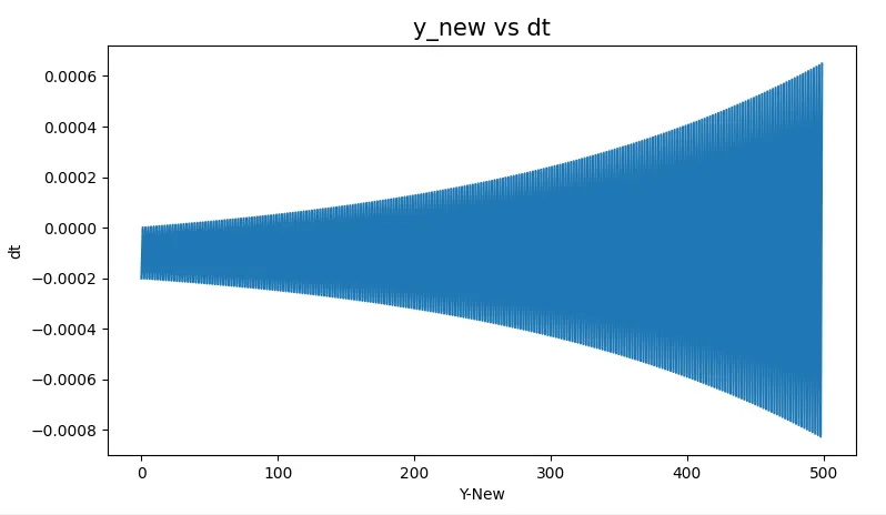
From this plot we can see that this is a unstable plot. As t_end and n values are changes we get the change in plot. Error of the ODE is depends upon t_end & n values. If we increase the n-values beyond 500, we get reverse plot.

As we used here backward differencing formula and Explicit method we get unstable solutions. So, from this we can conclude that explicit methods is more unstable than implicit methods.

2. Explicit Vs Implicit plot :-

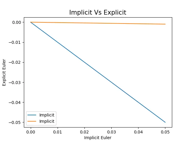
From above plot we can conclude that, Explicit gives stable solutions at any value while implicit is changes, as change in dt & coefficient of dt.

In both the method I solve backward differencing method and find out the stability as shown in above figure. As end time increases dt values decreases. In explicit method we can’t find out error easily but in implicit method we can find out error easily because error is directly depends upon dt value. If dt value increases error also increases and vice versa. In real world Implicit is a useful and important methods.

Q.1 :- When does a ODE becomes unstable ?

ANS. :- The answer of this question is in code-1. In that code we can observe that ODE depends upon t_end and number of points i.e. “n”. If either one changes then we get different solutions. If range beyond the normal range of t_end & n, then we getunstable solutions. Normally ODE becomes unstable for Explicit Euler methods.

Q.2 :- How does stability affect engineering simulations ?

ANS. :- Stability provides superior and good solutions to any simulations. If the stability maintains to any equations or simulations the error should be the minimum. Every research ongoing for the stabilizations of that simulations. Once simulations stabilize we get exact solutions with very least error.

Stability of solutions is important in physical problems because if slight deviation from the mathmatical model caused by unavoidable errors in measurment do not have a correspondingly slight effect on the solution, the mathmatical equations describing the problem will not accurately predict the future outcome. Thus, one of the difficulties in predicting populations growth is the fact that it is governed by the equation y = ax^ce, which is an unstable solution of the equation y’ =ay. Relatively slight errors in the initial populations count,c, or in the breeding rate, a, will cause quite large errors in predictions, even if no disturbing influences occur.

Q.3 :- Can stability condition be derived for all types of problem ?

ANS. :- Obviously Yes, Stability in mathmatics, condition in which a slight disturbances in a system does not produce too disrupting an effect on that system. In terms of the solution of a differential equation, a function f(x) is said tobe stable if any other solution of the equation that starts out sufficiently close to it when x=0 remains close to it for succeeding values of x. If the difference between the solutions approaches zero as x increases, the solution is called asymptotically stable. If a solution does not have either of these proparties, it is called unstable.

CONCLUSIONS :-

From above code and plots we can conclude following points are-

From above code and plots we can conclude following points are-

1. Stability of the ODE’s is depends upon the number of points used in the solution range.

2. An ODE’s error is directly proportional to the value of “dt”. If dt is more then error will more and vice versa.

3. Explicit methods remains constant for all solutions while implicit methods remaind stable for all solutions.

4. Due to above reason Implicit method is better than explicit methods.

5. In both the methods we can use backward differencing method easily.

6. For varifications of solutions and graph for any ODE’s we can use WolframAlpha keyboard which is official computational intelligence side.

7. Stability is most important for every ODE’s and we can apply it.

In this way I completed this project by writing code for two different examples, find out the plot, writing the results and finally write down the conclusions.