Numerical Integration techniques for solving ODEs and their stability issues.

AIM – Study the different numerical methods for solving ODEs to understand the stability issues in the solvers.

Ordinary Differential Equations (ODEs) –

Differential equations are among the most important mathematical tools used in producing models in the physical sciences, biological sciences, and engineering. The differential equations we consider are of the form

`y^' (t)=f(t,y(t))`

where y is the dependent variable and t is the independent variable. y(t) is the unknown function that is being sought. The given function f(t, y) of two variables defines the differential equation. This equation is called a first-order differential equation because it contains a first-order derivative of the unknown function, but no higher-order derivative.

The numerical methods for a first-order equation can be extended in a straightforward way to a system of first-order equations. Moreover, a higher-order differential equation can be reformulated as a system of first-order equations.

Solving ordinary differential equations –

Simple ordinary differential equations can be easily solved using hand calculations, however, for engineering applications, the ODEs are too complex to solve in such a way. Thus, numerical methods are used to solve the ODEs or a system of coupled ODEs. The reasons for use of numerical methods are –

1. More computational efforts are involved in Picard and Taylor series methods for complex real life applications
2. Easy availability of computers
3. The numerical methods can still be applied in cases where the closed form expression for the function is not available, but the values of function f are known at finitely many discrete points. The analytical methods are not applicable.

For example, the velocity of a particle is measured at given points and one is interested to predict the position of particle at some times in future. In such cases the analytical methods cannot be applied and one has to obtain solution by numerical methods.

Solution Methods -

Generally numerical methods are categorized in the following two categories –

1. Explicit Method
2. Implicit Method

Explicit methods utilize the current time step values to calculate the solution at the next time step. Forward Euler’s method, Runge Kutta Method of 4^th order are two examples of this method.

The advantage of this method is these are very easy to implement. However, a critical limitation is the stability issues observed. These methods are highly dependent on the time step size. While these methods will always give a result, the correctness of the result highly depends on the time step size. For large values of time step size, the solution becomes unstable and gives erroneous values. Using very small time step sizes is also not feasible due to increase in computation times.

Implicit methods are unconditionally stable. It must be noted that the solution might be stable but accuracy still depend on the time step size chosen. There solution doesn’t depend on the time step size. Thus, if converged, the implicit methods guarantee a correct solution. However, there implementation in a computer program is slightly difficult when compared to explicit methods. Backward Euler’s method is an example of implicit method.

Forward Euler Methods for solving ODEs –

This is the most basic method. It is not very practical to use for complex cases due to stability issues, however, it provides a very good starting point to use this method. It is a one-step method.

The numeric values of the solution y=g(t) are obtained at finitely many (say n) discrete points in the interval of interest. Let these n points be equi-spaced in the interval [t_o, b] as t₁, t₂, t₃ ….. t_n such that t = t_o + k_h , k = 1,2,...n. These points are known as grid points. Here the step size h is computed as

`h=(b-t_o)/n`

The numeric value of the solution is known at t=t_o. The approximate numeric value y_k of the solution at kth grid point t=t_k is an approximation to the exact solution y (t_k) of initial value problem (IVP). The Euler method specifies the formula for computing the solution:

The solution algorithm is –

1. Initialization – k = 0, `h=(b-t_o)/n`, y(t_k) = y_k
2. Computation

`y_(k+1)=y_k+hf(t_k,y_k )`

3. Increment – t_k+1 = t_k + h ; k = k+1
4. Check for continuation , if k
5. Stop

The above algorithm has been incorporated in a Python program for better understanding of the solution procedure for the ODE

`3y^'=t-y`

`y(0)=1`

Since this is a simple ODE, its analytical solution is

`y(t)=4 exp⁡(-t/3)+t-3`

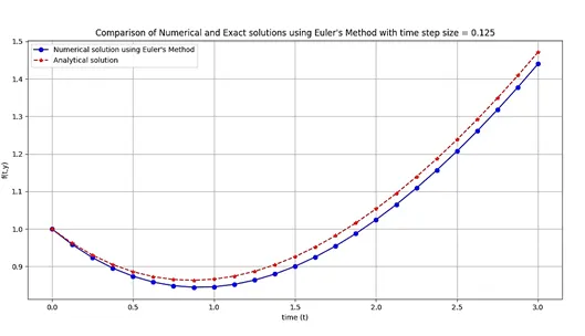
The results of the solution when h = 0.125 and function is evaluated between [0,3] is given in the below table –

k	t	yk	Exact Value	Error
0	0	1.00000	1.00000	0.00000
1	0.125	0.95833	0.96176	0.00342
2	0.25	0.92361	0.93018	0.00657
3	0.375	0.89554	0.90499	0.00944
4	0.5	0.87385	0.88593	0.01207
5	0.625	0.85828	0.87275	0.01447
6	0.75	0.84856	0.86520	0.01665
7	0.875	0.84445	0.86307	0.01862
8	1	0.84572	0.86613	0.02040
9	1.125	0.85215	0.87416	0.02201
10	1.25	0.86352	0.88696	0.02344
11	1.375	0.87962	0.90435	0.02472
12	1.5	0.90026	0.92612	0.02586
13	1.625	0.92525	0.95211	0.02686
14	1.75	0.95441	0.98214	0.02773
15	1.875	0.98756	1.01605	0.02849
16	2	1.02454	1.05367	0.02913
17	2.125	1.06518	1.09486	0.02968
18	2.25	1.10934	1.13947	0.03013
19	2.375	1.15687	1.18736	0.03049
20	2.5	1.20762	1.23839	0.03077
21	2.625	1.26147	1.29245	0.03098
22	2.75	1.31829	1.34940	0.03111
23	2.875	1.37794	1.40913	0.03119
24	3	1.44032	1.47152	0.03120

The same data obtained above can be represented graphically as shown below –

Python code for the above ODE -

"""
Program to solve an ODE using Euler Method
"""
import matplotlib.pyplot as plt
import math 
import numpy as np 

t_start = 0
t_end = 3
dt = 0.125

n = int((t_end-t_start)/dt) 	#to calculate the number of points

t_plot = np.linspace(t_start,t_end,n+1)	#For plotting the results

def f(t,y):		#y' = t/3 - y/3
	return t/3-y/3

def f_an(t):	#Analytical solution y = 4exp(-t/3)+t-3
	return 4*math.exp(-t/3)+t-3

t = t_start
y_0 = 1		#Initial value of y at t=t_start
y = y_0*np.ones(n+1)
y_analy = np.ones(n+1)

for k in range(0,n):
	y[k+1] = y[k] + dt*f(t,y[k])
	t = t+dt
	y_analy[k+1] = f_an(t)	#Doesn't calculate y[0]. It stores this value based on the initial condition. Elsewise we would have to define another loop for the same

err = y_analy-y
for i,j,k in zip(y,y_analy,err):
	print (i,j,k)
plt.plot(t_plot,y,'bo-')
plt.plot(t_plot,y_analy,'r*--')
plt.grid('on')
plt.legend(["Numerical solution using Euler's Method",'Analytical solution'])
plt.show()

It can be observed from the results above that the error between the numerical and exact solution. There are two reasons for this –

1. The solution is assumed to be of constant slope equal to f(t0,y0) in the interval (t0,t1)
2. Rounding errors in numerical computation of the formula.

The Final Global Error (F.G.E) in computing the final value at the end of the interval (a, b); a= t0, b=to+Mh is accumulated error in M steps and is of order h.

Apart from the Euler method, there are numerous numerical methods for solving IVP. These are not exhaustive. The selection of methods is based on the fact that these are generally used by scientists and engineers in solving IVP because of their simplicity. Also, more complex techniques are the combination of one or more of these and their development is on similar lines.

Stability analysis of Explicit and Implicit methods –

A general linear first order ODE is given as –

`y^'+ay+z=0`

Where a> 0 and z =z(t)`-1<1-aΔt<1`

1. Solving the above equation using Forward Euler’s method (Explicit) –

Expanding the derivative term using forward differencing method

`(y_(k+1)-y_k)/(Δt)= -ay_k-z_k`

`y_(k+1)=(1-aΔt) y_k-Δtz_k`

This form can easily be used to create an explicit Euler solver in any programming language.

The above equation can also be written as

`y_(k+1)=(1-aΔt)^(k+1) y_0-Δtz_k`

For the solution to be decaying (stable)

`|1-aΔt|<1`

`-1<1-aΔt<1`

This gives

`aΔt>0 and`

`Δt<2/a`

Thus, the stability of the Forward Euler’s Method is dependent on both a and ∆t.

2. Solving the ODE using Backward Euler’s method (Implicit) –

Expanding the derivative term using forward differencing method

`(y_(k+1)-y_k)/(Δt)= -ay_(k+1)-z_(k+1)`

`y_(k+1)=1/(1+aΔt) y_k-(Δt)/(1+aΔt) z_(k+1)`

This form can easily be used to create an implicit Euler solver in any programming language.

The above equation can also be written as

`y_(k+1)=(1/(1+aΔt))^(k+1) y_0-(Δt)/(1+aΔt) z_(k+1)`

For the solution to be decaying (stable)

`|1+aΔt|>1`

Since a and ∆t are always greater than zero, the above condition always holds.

To get a clearer picture of the stability issues in the solution of an ODE when using explicit methods, consider the following ODE

`f(t,y)= y^'= -1000y-exp⁡(-t)`

The exact solution of the above differential equation is

`y=(exp⁡(-1000t)*(1-exp⁡(999t)))/999`

The above ODE is solved numerically using Python and the results obtained are given below.

A general ODE slver has been developed for such ODEs -

Driver code -

from ODESolver import *
import math
import numpy as np

#Driver Script

t_start = 0
t_end = 0.1
dt = 20e-4
y0 = 0
"""
y' + a(t)y(t) + z(t) = 0
where y = f(t,y)
y' = dy/dt
a = a(t)
z = z(t)


ODEEuler(f,t_start,t_end,dt,y0)
y'+ ay + z = 0
z - needs to ebe explicitly defined while defining f
f - Function to be solved (y') = -z-ay
"""
a = 1000
#z = lambda t:-math.exp(-t)
f = lambda t,y:-math.exp(-t)-a*y
y_eul_exp,n = ODEEulerExplicit(f,a,t_start,t_end,dt,y0)
y_eul_imp,n = ODEEulerImplicit(f,a,t_start,t_end,dt,y0)

#Analytical solution of the function f in the above line
y_analy = np.ones(n+1)
t = np.linspace(t_start,t_end,n+1)
for i in range(0,n+1):	#range function excludes end point. Thus to access t[end] we deifine range(0,n+1)
	y_analy[i] = np.exp(-1000*t[i])*(1-np.exp(999*t[i]))/999

plt.plot(t,y_eul_exp)
plt.plot(t,y_eul_imp)
plt.plot(t,y_analy,'--')
plt.grid('on')
plt.title("Comparison of Exact and Numerical solution with time step size = {0}".format(dt))
plt.xlabel('time (t)',fontsize = 12)
plt.ylabel('f(t,y)',fontsize = 12)
plt.legend(['Forwad Euler's Method (Explicit)','Backward Euler's Method (Implicit)','Analytical solution (Exact)'])
plt.show()

GENERAL ODE SOLVER (Forward and Backward Euler)

"""
Program to solve an ODE using Euler Method
"""
import matplotlib.pyplot as plt
import math 
import numpy as np 

"""
y' + a(t)y(t) + z(t) = 0
where y = f(t,y)
y' = dy/dt
a = a(t)
z = z(t)


ODEEuler(f,t_start,t_end,dt,y0)
y'+ ay + z = 0
z - needs to ebe explicitly defined while defining f
f - Function to be solved (y') = -z-ay


ODEEuler(f,a,t_start,t_end,dt,y0)

f - Function to be solved (y') = z-ay
t_start - start time of integration (lower limit)
t_end - End time of integration (upper limit)
dt - time step size
y0 - Initial value of y i.e. y at t=t_start
"""


def ODEEulerExplicit(f,a,t_start,t_end,dt,y0):
	if (t_start>=t_end):
		print('Integration lower limit must be smaller than upper limit')

	if(dt>=t_end or dt<=t_start):
		print('Incorrect time step size')
		
	n = int((t_end-t_start)/dt) 	#to calculate the number of points

	t = t_start
	y_0 = y0		#Initial value of y at t=t_start
	y = y_0*np.ones(n+1)
	print("ODEEulerExplicit() returns the value of function and number of points (n) using the Forward Euler's Methodnn")

	for k in range(0,n):
		y[k+1] = (1-a*dt)*y[k]+dt*f(t,0)	#Same as y[k+1] = y[k] + dt*f(t,y[k])
		t = t+dt

	return y,n

def ODEEulerImplicit(f,a,t_start,t_end,dt,y0):
	if (t_start>=t_end):
		print('Integration lower limit must be smaller than upper limit')
		
	if(dt>=t_end or dt<=t_start):
		print('Incorrect time step size')
		
	n = int((t_end-t_start)/dt) 	#to calculate the number of points

	t = t_start
	y_0 = y0		#Initial value of y at t=t_start
	y = y_0*np.ones(n+1)
	print("ODEEulerImplicit() returns the value of function and number of points (n) using the Backward Euler's Methodnn")

	for k in range(0,n):
		t = t+dt
		y[k+1] = (y[k]+dt*f(t,0))/(1+a*dt)	#Obtained after simplifying y[k+1] = y[k] + hf(t[k+1],y[k+1])
		
	return y,n

Results and Discussion –

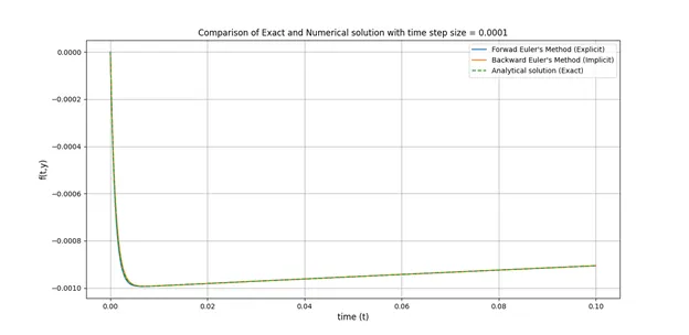
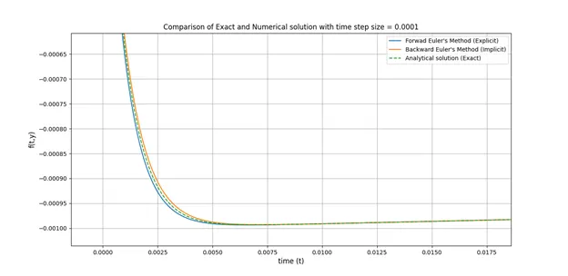
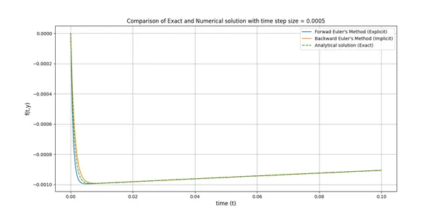
The solution of the above ODE at different time steps is shown in the below plots

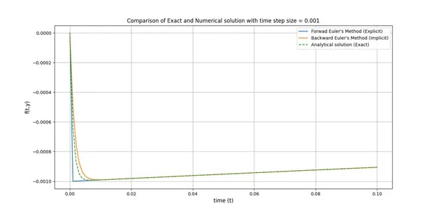
1. At time step = 0.0001, it can be observed from the zoomed in images that Forward Euler’s method under predicts the solution while Backward Euler’s Method over predicts it. In fact, there is an inherent error of the order of time step in both these methods. The accuracy can further be improved by reducing the time step.
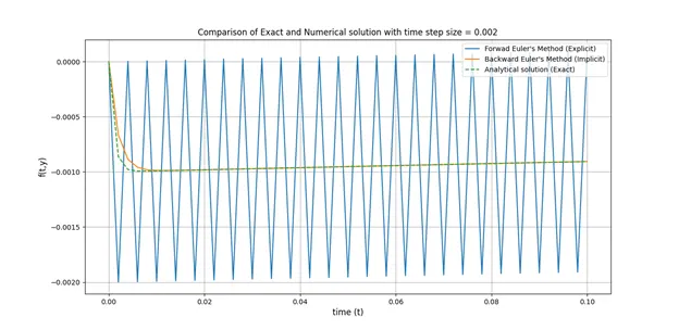
2. When the time step is increased from 1e-4 to 20e-4, it can be observed that the solution from the Forward Euler method starts diverging from the actual solution. The solution from the backward Euler’s method still follows the actual solution with only slight errors. This proves the major flaw in the Forward Euler Method.

Time Step	Stability condition (∆t<(2/a) i.e. ∆t<0.002) satisfied?
1e-4	Yes
5e-4	Yes
10e-4	Yes
20e-4	No

As it was proved earlier, that the Forward Euler method is conditionally stable for a>0. When time step is 20e-4, this stability condition is not followed and the solution becomes unstable.

Importance of stability –

Any numerical method being used must be stable. This will guarantee that the solution obtained is bounded and is reliable. In case, a proper method is not chosen, garbage values will be returned by the simulation and if relied upon, will lead to system failure in real life situation.

Thus, a proper compromise is needed between stability, accuracy and computational time taken. Implicit methods are unconditionally stable. However, these are slow and require higher computation times. Explicit methods although are fast but are conditionally stable.

Stability analysis of complex ODEs –

Stability analysis of any ODE is not possible since the mathematics becomes too complex. Thus, in such cases, implicit solvers are relied upon so that we get reliable and accurate solution of the equations.