Week 5 - Literature review: ODE Stability

1.When does a ODE become unstable?

Ans.For the explicit Euler method,stability condition is

`|1+h*lamda|<=1`

`lamda`=Coefficient in function

h=time step size

The explicit Euler method is called stable for the test equation (1) if the step size h satisfies

the condition.

In the case of real and negative λ,this means

`h<=-2/lamda`

##Here is the program giving proof of unstabe solution using Explicit Euler method and Implicit Euler method.

Consider the problem

Y'(x) = λY (x) + (1 − λ) cos(x) − (1 + λ) sin(x),Y(0)=1

The true solution is Y (x) = sin(x) + cos(x)

here λ=-10;

"""
Explicit and Implicit method for ODE

"""

import math
import matplotlib.pyplot as plt
import numpy as np


def f(total_t,dt,t):
	

	return math.sin(t[i])+math.cos(t[i])			#Analytical function f(t)-sin(t)+cos(t)


	




total_t=10											#Total time
dt=0.1											#Time step size



t=0
y_old=0												#Initial guess value of y ,denoted as y_old (for Euler explicit method)
t=np.arange(0,total_t,dt)							#Array of time step
y_new=np.zeros(len(t))								#Array of values of y in next time step,denoted as y_new

y_analy=np.zeros(len(t))


for i in range(0,len(t)):
	y_new[i]=y_old+dt*((11*math.cos(t[i]))+(9*math.sin(t[i]))-10*y_old)
	y_old=y_new[i]
	y_analy[i]=f(total_t,dt,t)						#y_analy ,calculating analytical value of given function f(t)



y_old1=0											#Initial guess value of y ,denoted as y_old1 (for Euler Implicit method)
y_new1=np.zeros(len(t))								#Array of values of y in next time step,denoted as y_new1

	
for i in range(0,len(t)):
	y_new1[i]=(y_old1+dt*((11*math.cos(t[i]))+(9*math.sin(t[i]))))/(1+10*dt)
	y_old1=y_new1[i]
	


print(dt)
plt.plot(y_new,color='red',label='Explicit')
plt.plot(y_new1,color='blue',label='Implicit')
plt.plot(y_analy,color='green',label='Analytical')
plt.legend(loc="lower left")

plt.show()

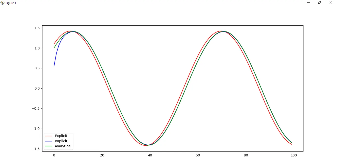
The above plot is for dt=0.1 sec and total time=10sec,which is in the stability range.Plot also show after certain time period all three solution are coincident.

----------------------------------*******************************---------------------------------------

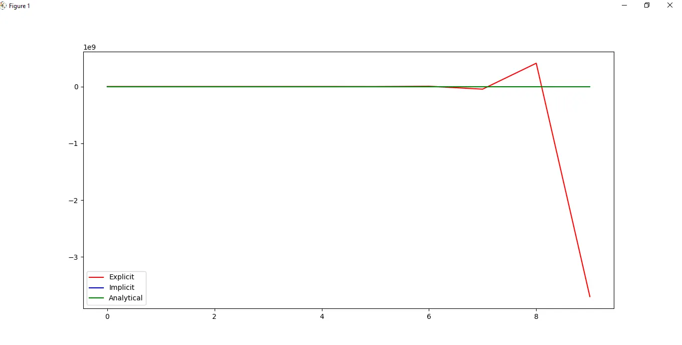
##Below plot is for t=1 and total time=10,which is out of stability range.Plot show Analytical and Implicit solution folows each other but Explicit solution deviating and giving absurd results.

------------------------------***********************************-------------------------------------

2.How does stability affect engineering simulations?

Ans.Like engineering simulation talking about fluid mechanics gives a solution by converting complex coupled partial differential equation into linear algebric equations through discritisation.For discritisation also mainly now a days FVM is used.It also uses various schemes like First order upwind,Second order upwind,etc.

Stability in engineering simulations depends on some factors like schemes named above,time step size,mesh grid size,relaxation factor.

Like if we used coarse mesh with fist order upwind scheme,we will get converged solution fast but it would not be accurate and stable.So if mesh is coarse choosing second order scheme is a good choice.Second order scheme use more number of neighbouring cells to computes flow variables at a point,therefore it gives accurate results.

Under relaxation factor also helps in giving solution greater stability,means it will take more time in convergence as compared to solution where system is not relaxed or over relaxed.Under relaxation factor prevents oscilation in our results.

Courant number ,it also affect simulation results.This term gives unstable results if size of our time step is larger than the distance between two neighbouring cells in mesh grid.So using correct time step size is very important in some cases.

------------------------------------********************************------------------------------------

3.Can stability condition be derived for all types of problems?

Ans.No stability condition cannot be derived for all types of problems.

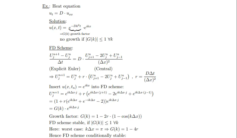
But von neumann stability and linear stability analysis can help in deriving stability conditions for various problems.

#By von neumann stability

#Linear stability:

In mathematics, in the theory of differential equations and dynamic systems, a particular stationary or quasistationary solutionto a nonlinear system is called linearly unstable if the linearizationof the equation at this solution has the form,

`(dr)/(dt)=Ar`

where A is a linear operator whose spectrum contains eigenvalues with positive real part. If all the eigenvalues have negative real part, then the solution is called linearly stable. Other names for linear stability include exponential stability or stability in terms of first approximation.