Literature review: ODE Stability

AIM

The aim is to conduct a literature review on stability of ODE

STABILITY OF ODE

In mathematics, stability theory addresses the stability of solutions of ODE and of trajectories of dynamical systems under small perturbations of initial conditions. The heat equation, for example, is a stable partial differential equation because small perturbations of initial data lead to small variations in temperature at a later time as a result of the maximum principle. In partial differential equations one may measure the distances between functions using LD norms or the sup norm, while in differential geometry one may measure the distance between spaces using the Gromov's Distance.

In dynamical systems, an orbit is called Lyapunov stable if the forward orbit of any point is in a small enough neighbourhood or it stays in a small (but perhaps, larger) neighbourhood. Various criteria have been developed to prove stability or instability of an orbit. Under favourable circumstances, the question may be reduced to a well-studied problem involving eigen values of matrices.

Now let’s define a simple ODE

`dx /dt = f(x)`

Now if we take the stability for this equation, it can be assumed that the solution is stable at `dx/dt = 0`

The initial conditions for ODE decides the stability of the equation

If x(o) = `x_0` , x(t) = `x_0`

if x(0) = `x_1`, which is close to `x_0``x_1nex_0`

When x(t) approaches x_0 we say the solution is converging and meeting a specific value. This indicates the solution is stable. But when x(t) deviates from this point we say that the solution is becoming unstable.

PYTHON CODE FOR STABILITY OF ODE

Lets take an example to explain stability

`dy/dt = -10000*y - exp(-t)`

Solving the equation in explicit fashion, we obtain

`y^(n+1) = y^n -10000*y^n*Delta(t) - exp(-t)*Delta(t)`

Now it can be also solved in implicit scheme as below

`y^n = (y^(n-1) -exp(-t).Delta(t))/(1 + 10000*Delta(t)`

The analytical solution is obtained as follows

`y(t) = (e^(-10000 t) (1 - e^(9999 t)))/9999`

import matplotlib.pyplot as plt
import numpy as np

def explicit_euler(total_t, dt):
	t = np.arange(0, total_t, dt)
	y = np.zeros(len(t))

	for i in range(1, len(t)):
		y[i] = y[i-1] + dt*(-10000*y[i-1] - np.exp(-t[i-1]));

	return (t,y)

def implicit_euler(total_t,dt):
	t = np.arange(0, total_t,dt)
	y = np.zeros(len(t))

	for i in range(1,len(t)):
		y[i] = (y[i-1] - np.exp(-t[i-1])*dt)/(1-10000*dt);

	return (t,y)
def analytical(total_t, dt):
	t = np.arange(0, total_t,dt)
	y = np.zeros(len(t))

	for i in range(1,len(t)):
		y[i] = np.exp(-10000*t[i]) * (1- np.exp(9999*t[i]))/9999;
	return y


	
total_t = 0.1
dt = 1e-4
t,y_explicit = explicit_euler(total_t,dt)
t,y_implicit = implicit_euler(total_t,dt)
y_analytical = analytical(total_t,dt)
plt.plot(t,y_explicit)
plt.plot(t,y_implicit)
plt.plot(t,y_analytical)
plt.legend(['Explicit','Implicit','Analytical'])
plt.show()

Now in this code we are defining three functions of explicit, implicit and analytical solution for the example differential equation which is considered for this case. Now we define t and y as arrays and then by using for statements we define the formulas for the various methods and then the results are plotted for comparison

Now in order to obtain a solution for the ODE we have to select the appropriate time steps which is shown below

CODE OUTPUT(dt = 1e-4)

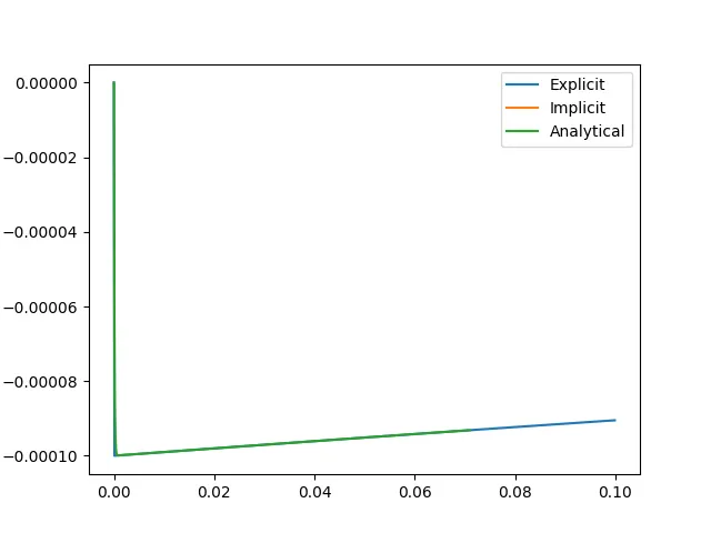
This plot shows that all the three solutions are in good match with the analytical solution

CODE OUTPUT(dt = 1e-3)

CODE OUTPUT(dt = 1e-2)

CODE OUTPUT(dt = 5e-2)

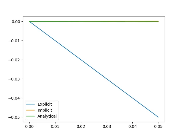
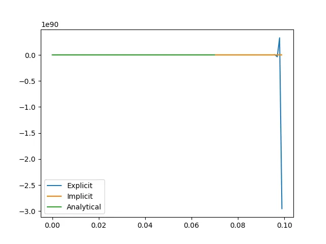
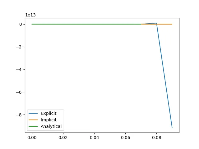
From the above plots we see that the explicit scheme starts to oscillate when the time step starts increasing from 1e-4. The solution then blows up which gives all wrong answers for the solution of the ODE. The time step in the major factor which decides if the solution is stable or not. Usually the stability criteria needs to be derived only for explicit schemes but implicit schemes are quite stable. The implicit scheme does not involve the derivation of any stability criteria.

CONCLUSION

1. ODE becomes unstable with explicit scheme or when solution diverges from equilibrium point
2. Implicit schemes are quite stable at wide range of time step values.
3. The stability criteria helps widely for engineering simulations if it is derived for explicit scheme
4. There is no necessity for stability for implicit scheme.