Week 5 - Genetic Algorithm
GENETIC ALGORITHM
Genetic algorithms are a type of optimization algorithm, meaning they are used to find the optimal solution(s) to a given computational problem that maximizes or minimizes a particular function. Genetic algorithms represent one branch of the field of study called evolutionary computation, in that they imitate the biological processes of reproduction and natural selection to solve for the fittest solutions.
In computer science and operations research, a genetic algorithm (GA) is a metaheuristic inspired by the process of natural selection that belongs to the larger class of evolutionary algorithms (EA). Genetic algorithms are commonly used to generate high-quality solutions to optimization and search problems via biologically inspired operators such as selection, crossover, and mutation.
The basic components common to almost all genetic algorithms are :
- A fitness function for optimization
- A population of solutions
- Selection of which solutions will regenerate
- Crossover to generate next generation of solutions
- Random mutation of solutions in new generation
Fitness Function –
A fitness function value quantifies the optimality of a solution. The value is used to rank a particular solution against all the other solutions. A fitness value is assigned to each solution depending on how close it is to the optimal solution of the problem.
Population –
The major questions to consider are firstly the size of the population, and secondly the method by which the individuals are chosen. The size of the population has been approached from several theoretical points of view, although the underlying idea is always of a trade-off between efficiency and effectiveness. Intuitively, there should be some ‘optimal’ value for a given string length, on the grounds that too small a population would not allow sufficient room for exploring the search space effectively, while too large a population would so impair the efficiency of the method that no solution could be expected in a reasonable amount of time.
Selection –
The primary objective of the selection operator is to emphasize the good solutions and eliminate the bad solutions in a population while keeping the population size constant.
Crossover –
The crossover operator is used to create new solutions from the existing solutions available in the population pool after applying selection operator. This operator exchanges the string information between the solutions in the population pool.
Mutation –
Mutation is the occasional introduction of new features into the solution strings of the population pool to maintain diversity in the population. Though crossover has the main responsibility to search for the optimal solution, mutation is also used for this purpose.
Advantages of GAs -
- Does not require any derivative information (which may not be available for many real-world problems).
- Is faster and more efficient as compared to the traditional methods.
- Has very good parallel capabilities.
- Optimizes both continuous and discrete functions and multi-objective problems.
- Provides a list of “good” solutions and not just a single solution.
- Always gets an answer to the problem, which gets better over the time.
- Useful when the search space is very large and there are a large number of parameters involved.
Limitations of GAs -
- GAs are not suited for all problems, especially problems which are simple and for which derivative information is available.
- Fitness value is calculated repeatedly which might be computationally expensive for some problems.
- Being stochastic, there are no guarantees on the optimality or the quality of the solution.
- If not implemented properly, the GA may not converge to the optimal solution.
CODE TO OPTIMIZE STALAGMITE FUNCTION AND FIND THE GLOBAL MAXIMA OF THE FUNCTION
Syntax used in this project –
1. [x,fval] = ga(___)
- for any previous input arguments, also returns fval, the value of the fitness function at x.
2. [x,fval] = ga(fun,nvars,A,b,Aeq,beq,lb,ub)
- defines a set of lower and upper bounds on the design variables, x, so that a solution is found in the range lb ≤ x ≤ ub. (Set Aeq=[] and beq=[] if no linear equalities exist.)
3. [x,fval] = ga(fun,nvars,A,b,Aeq,beq,lb,ub,nonlcon,options)
- minimizes with the default optimization parameters replaced by values in options. (Set nonlcon=[] if no nonlinear constraints exist.) Create options using optimoptions.
Stalagmite Function Syntax –
function [Fxy]=stalagmite_func(inpt_vctr)
f1x=(sin(((5.1*pi).*inpt_vctr(1))+0.5)).^6;
f2x=exp((-4*log(2)*(inpt_vctr(1)-0.0667).^2)/0.64);
f1y=(sin(((5.1*pi).*inpt_vctr(2))+0.5)).^6;
f2y=exp((-4*log(2)*(inpt_vctr(2)-0.0667).^2)/0.64);
[F_xy]=(f1x*f2x*f1y*f2y);
[Fxy]=-F_xy; % TO COMPUTE LOCAL MAXIMA USING GA
end
Matlab Script Syntax –
clear
close all
clc
% CODE TO FIND GLOBAL MAXIMA USING GA FOR STALAGMITE FUNCTION
% GENERATING ONE DIMENSIONAL VECTORS
x=linspace(0,0.7,151);
y=linspace(0,0.7,151);
% DETERMINE NUMBER OF ITTERATIONS FOR GA
num_itt=51;
% GENERATING TWO DIMENSIONAL VECTORS
[xx,yy]=meshgrid(x,y);
% NESTED LOOPS TO COMPUTE STALAGMITE FUNCTION WITH INPUT VECTORS
for i=1:length(xx)
for j=1:length(yy)
inpt_vctr(1)=xx(i,j);
inpt_vctr(2)=yy(i,j);
f(i,j)=stalagmite_func(inpt_vctr);
end
end
% GENERATING SURFACE PLOT OF STALAGMITE FUNCTION
figure(1)
surfc(-xx,-yy,-f)
shading interp
hold on
xlabel('X-values');ylabel('Y-values');zlabel('Function-values')
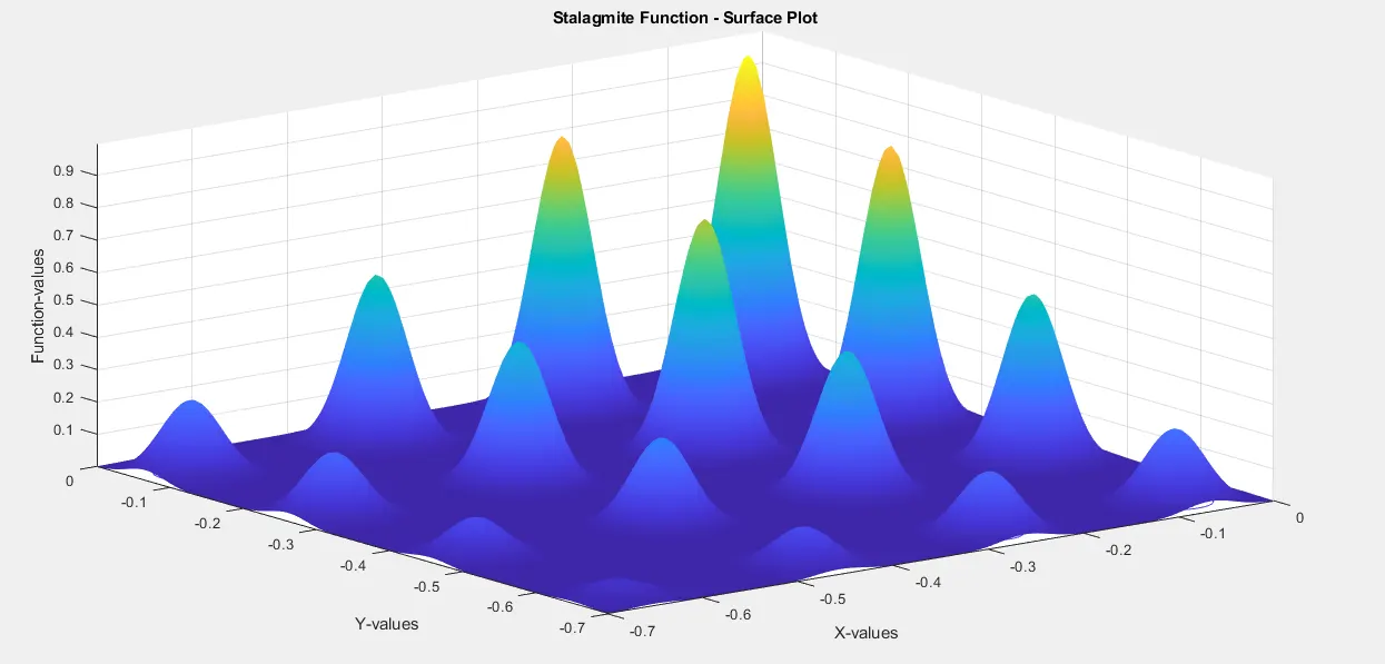
title('Stalagmite Function - Surface Plot')
hold off
%% CASE STUDY-1 : UNCONSTRAINED FUNCTION MAXIMA
tic
for k=1:num_itt
[f1_inpt,f1_otpt(k)]=ga(@stalagmite_func,2);
x1_inpt(k)=f1_inpt(1);
y1_inpt(k)=f1_inpt(2);
end
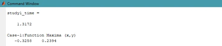
study1_time=toc
figure(2)
subplot(2,1,1)
surfc(-x,-y,-f)
shading interp
hold on
plot3(-x1_inpt,-y1_inpt,-f1_otpt,'marker','o','markersize',4,'markerfacecolor','r')
xlabel('X-values');ylabel('Y-values');zlabel('Function-values')
title('Case-1:Unconstrained Function Values');hold off
subplot(2,1,2)
plot(-f1_otpt)
xlabel('Number of Itterations');ylabel('Function Values')
title('Itterations vs Function Maxima')
disp('Case-1:Function Maxima (x,y)')
disp(f1_inpt)
%% CASE STUDY-2 : CONSTRAINED FUNCTION MAXIMA
tic
for k=1:num_itt
[f2_inpt,f2_otpt(k)]=ga(@stalagmite_func,2,[],[],[],[],[0;0],[1;1]);
x2_inpt(k)=f2_inpt(1);
y2_inpt(k)=f2_inpt(2);
end
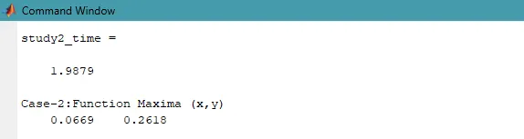
study2_time=toc
figure(3)
subplot(2,1,1)
surfc(-x,-y,-f)
shading interp
hold on
plot3(-x2_inpt,-y2_inpt,-f2_otpt,'marker','o','markersize',4,'markerfacecolor','r')
xlabel('X-values');ylabel('Y-values');zlabel('Function-values')
title('Case-2:Constrained Function Values');hold off
subplot(2,1,2)
plot(-f2_otpt)
xlabel('Number of Itterations');ylabel('Function Values')
title('Itterations vs Function Maxima')
disp('Case-2:Function Maxima (x,y)')
disp(f2_inpt)
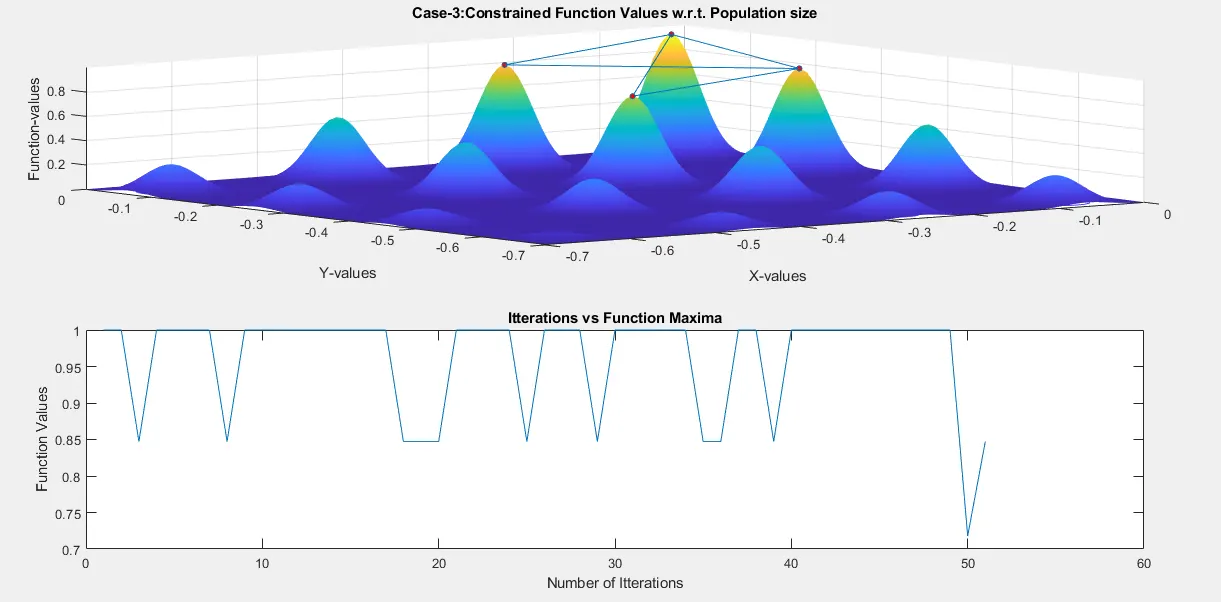
%% CASE STUDY-3 : CONSTRAINED FUNCTION MAXIMA WITH POPULATION SIZE
% GENERATE POPULATION TO CONSTRAIN FUNCTION WITHIN POPULATION SIZE
% USING "OPTIMOPTIONS" TO DEFINE POPULATION SIZE
options1=optimoptions('ga','populationsize',101);
tic
for k=1:num_itt
[f3_inpt,f3_otpt(k)]=ga(@stalagmite_func,2,[],[],[],[],[0;0],[1;1],[],[],options1);
x3_inpt(k)=f3_inpt(1);
y3_inpt(k)=f3_inpt(2);
end
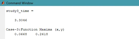
study3_time=toc
figure(4)
subplot(2,1,1)
surfc(-x,-y,-f)
shading interp
hold on
plot3(-x3_inpt,-y3_inpt,-f3_otpt,'marker','o','markersize',4,'markerfacecolor','r')
xlabel('X-values');ylabel('Y-values');zlabel('Function-values')
title('Case-3:Constrained Function Values w.r.t. Population size');hold off
subplot(2,1,2)
plot(-f3_otpt)
xlabel('Number of Itterations');ylabel('Function Values')
title('Itterations vs Function Maxima')
disp('Case-3:Function Maxima (x,y)')
disp(f3_inpt)
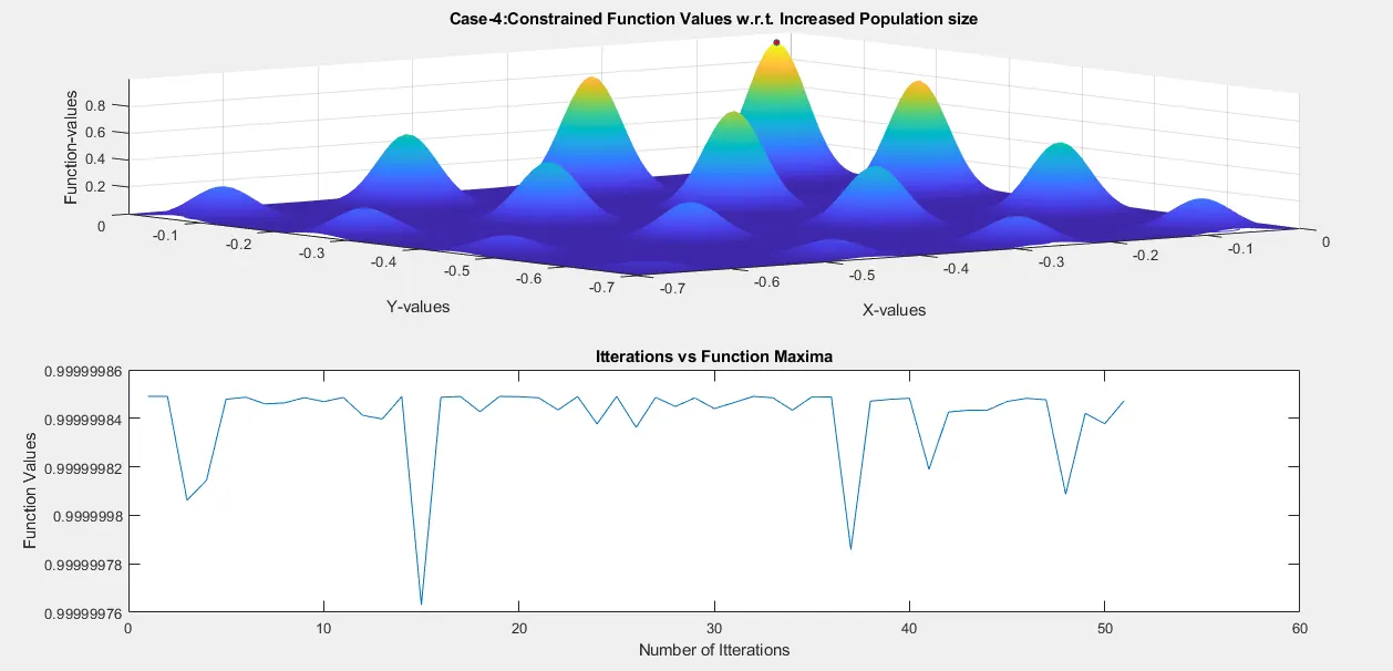
%% CASE STUDY-4 : CONSTRAINED FUNCTION MAXIMA WITH INCREASED POPULATION SIZE
% INCREASING POPULATION TO CONSTRAIN FUNCTION WITHIN POPULATION SIZE
% USING "OPTIMOPTIONS" TO DEFINE POPULATION SIZE
options2=optimoptions('ga','populationsize',401);
tic
for k=1:num_itt
[f4_inpt,f4_otpt(k)]=ga(@stalagmite_func,2,[],[],[],[],[0;0],[1;1],[],[],options2);
x4_inpt(k)=f4_inpt(1);
y4_inpt(k)=f4_inpt(2);
end
study4_time=toc
figure(5)
subplot(2,1,1)
surfc(-x,-y,-f)
shading interp
hold on
plot3(-x4_inpt,-y4_inpt,-f4_otpt,'marker','o','markersize',4,'markerfacecolor','r')
xlabel('X-values');ylabel('Y-values');zlabel('Function-values')
title('Case-4:Constrained Function Values w.r.t. Increased Population size');hold off
subplot(2,1,2)
plot(-f4_otpt)
xlabel('Number of Itterations');ylabel('Function Values')
title('Itterations vs Function Maxima')
disp('Case-4:Function Maxima (x,y)')
disp(f4_inpt)
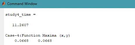
Output - Command Window
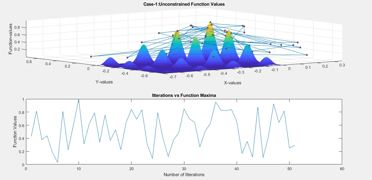
CASE STUDY-1 : UNCONSTRAINED FUNCTION MAXIMA
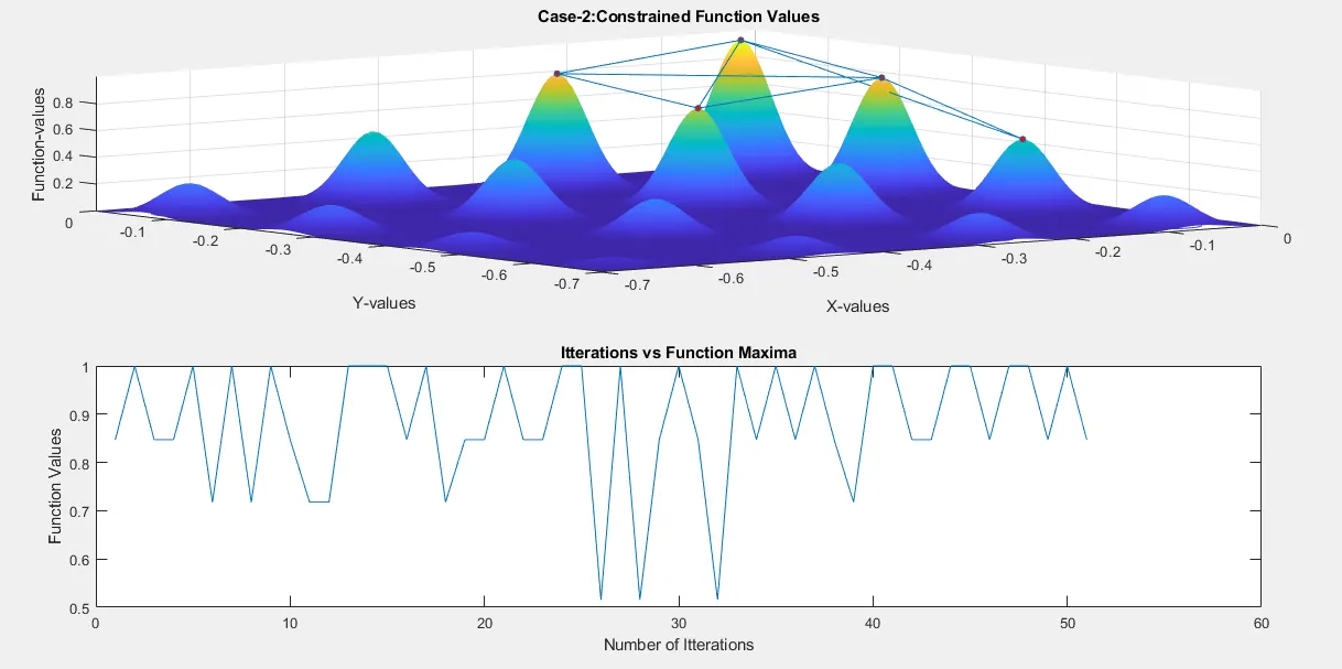
CASE STUDY-2 : CONSTRAINED FUNCTION MAXIMA
CASE STUDY-3 : CONSTRAINED FUNCTION MAXIMA WITH POPULATION SIZE
CASE STUDY-4 : CONSTRAINED FUNCTION MAXIMA WITH INCREASED POPULATION SIZE
Output - Figures
STALAGMITE FUNCTION PLOT
CASE STUDY-1 : UNCONSTRAINED FUNCTION MAXIMA
CASE STUDY-2 : CONSTRAINED FUNCTION MAXIMA
CASE STUDY-3 : CONSTRAINED FUNCTION MAXIMA WITH POPULATION SIZE
CASE STUDY-4 : CONSTRAINED FUNCTION MAXIMA WITH INCREASED POPULATION SIZE