Week 5 - Genetic Algorithm

Function Script:

 

function [S] = stalagmite(input_vector)

x = input_vector (1); 
y = input_vector (2);

f1_x = (sin(5.1*pi * x +0.5)).^6;
f2_y = (sin(5.1*pi * y +0.5)).^6;
f3_x = exp((-4*0.6931).*(x-0.0667)^2/(0.64));
f4_y = exp((-4*0.6931).*(y-0.0667)^2/(0.64));

s = (f1_x.*f2_y.*f3_x.*f4_y);
S = -s;

end

Defining Search Space:

close all
clc

%% Defining search space

x = linspace(0,0.6,150);
y = linspace(0,0.6,150);
num_cases = 50;

%%Creating 2D Mesh

[XX YY] = meshgrid(x,y);

%%Evaluating the stalagmite function

for i=1:length(XX)
    for j=1:length(YY)
        input_vector(1)= XX(i,j);
        input_vector(2)= YY(i,j);
        f(i,j) = stalagmite(input_vector);

    end
end

% Converting Fitting Function to change the graph upwards
F = -f;

% Plotting Stalagmite Function

surf(XX,YY,F);
shading interp;
hold on;

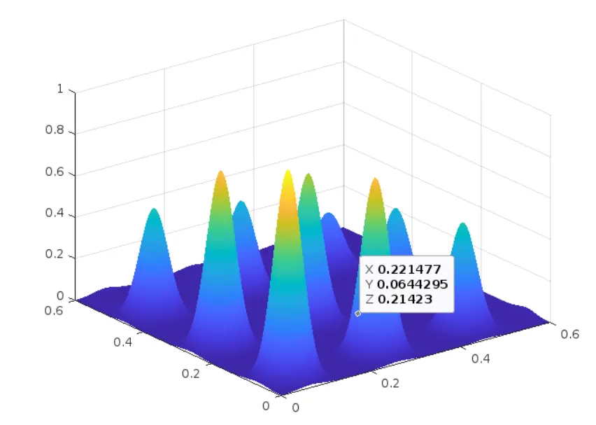
This script gives a visual representation of the search space of the function.

Performing Genetic algorithm with no bounds;

% Performing the Genetic Algorithm 1st Case

tic
for i = 1:num_cases
[inputs1,Fopt1(i)] = ga(@stalagmite,2);
xopt1(i) = inputs1(1);
yopt1(i) = inputs1(2);
end
study_time1 = toc;


figure(2)
subplot(2,1,1)
hold on
surfc(XX,YY,f)
shading interp
xlabel('X data')
ylabel('Y data')
plot3(xopt1,yopt1,Fopt1,'marker','o','markersize',5,'markerfacecolor','r');
title('Bounded Inputs')
subplot(2,1,2)
plot(Fopt1)
xlabel('Iterations')
ylabel(' Maximum Function')
hold off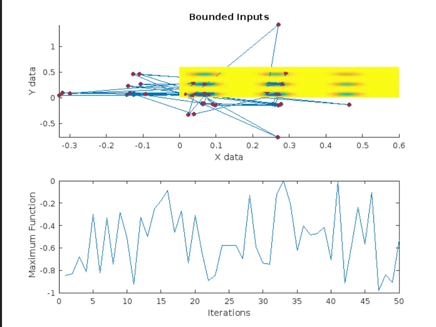

Observation:

Whenever we don't define any search space the result we get is random. We can't rely on the code to reach a conclusion. The range of iterations is almost 0 to -1 which is not reliable.

Performing GA with upper and lower bounds:

% Performing the Genetic Algorithm 2nd Case

tic
for i = 1:num_cases
[inputs2,Fopt2(i)] = ga(@stalagmite,2,[],[],[],[],[0;0],[0.6;0.6]);
xopt2(i) = inputs2(1);
yopt2(i) = inputs2(2);
end
study_time2 = toc;


figure(3)
subplot(2,1,1)
hold on
surfc(XX,YY,f)
shading interp
xlabel('X data')
ylabel('Y data')
plot3(xopt2,yopt2,Fopt2,'marker','o','markersize',5,'markerfacecolor','r');
title('Bounded Inputs')
subplot(2,1,2)
plot(Fopt2)
xlabel('Iterations')
ylabel(' Maximum Function')
hold off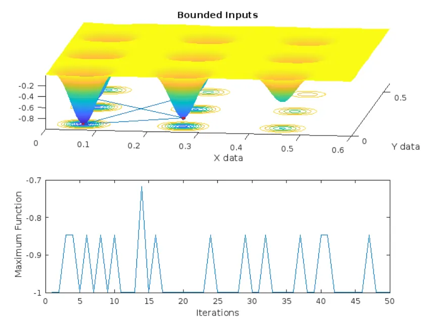

Observation:

Defining search space limits the random values somewhat. Still the range of iterations is almost -0.7 to -1 which is more that allowable limit.

Performing GA with Bounds and more population size:

% Performing the Genetic Algorithm 3rd Case

options = optimoptions('ga');
options = optimoptions(options,'populationsize',300);

tic
for i = 1:num_cases
[inputs3,Fopt3(i)] = ga(@stalagmite,2,[],[],[],[],[0;0],[0.6;0.6],[],[],options);
xopt3(i) = inputs3(1);
yopt3(i) = inputs3(2);
end
study_time3 = toc;


figure(4)
subplot(2,1,1)
hold on
surfc(XX,YY,f)
shading interp
xlabel('X data')
ylabel('Y data')
plot3(xopt3,yopt3,Fopt3,'marker','o','markersize',5,'markerfacecolor','r');
title('Bounded Inputs')
subplot(2,1,2)
plot(Fopt3)
xlabel('Iterations')
ylabel(' Maximum Function')
hold off

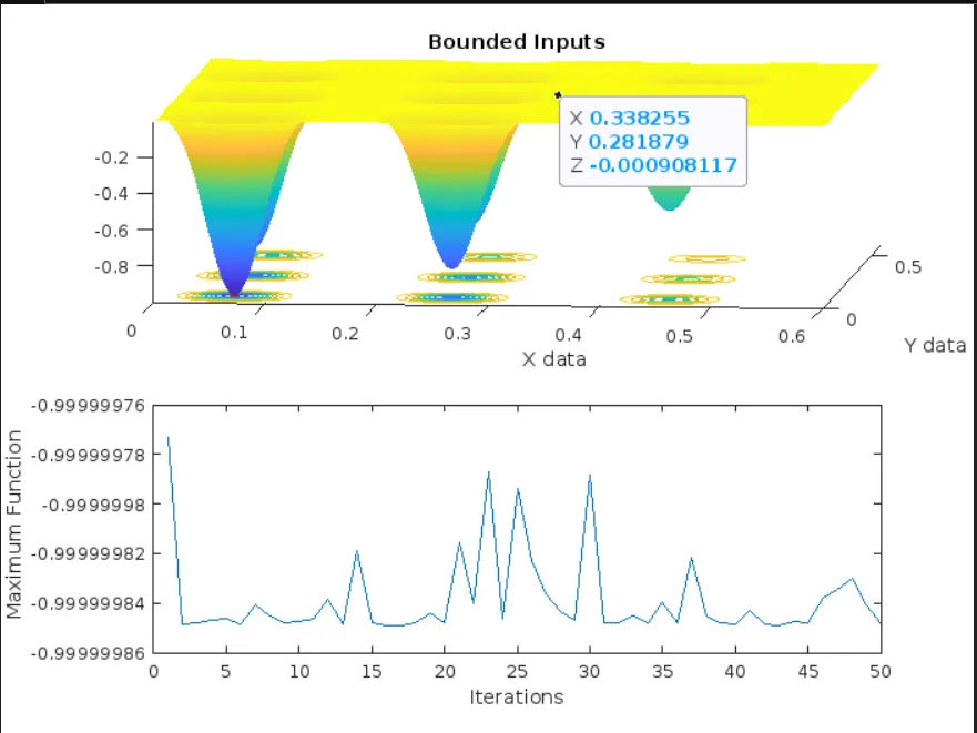
Observation:

When we increase population size besides bounding the limits we can rely on the code. We can see that the iteration range is very small and within the limit.