Week 5 - Genetic Algorithm

STALAGMITE FUNCTION

function [f] = stalagmite(input_vector)
    x = input_vector(1);
    y = input_vector(2);

    t1 = (sin((5.1*pi*x)+0.5))^6;
    t2 = (sin((5.1*pi*y)+0.5))^6;
    t3 = exp(-4*log(2)*((x-0.0667)^2)/0.64);
    t4 = exp(-4*log(2)*((y-0.0667)^2)/0.64);

    f = -(t1*t2*t3*t4);
end

GENERAL ALGORITHM FOR STALAGMITE FUNCTION

%clear all is clear all variables in the current workspace
%close all is for closing figures which are open
%clc is for clearing text in command window
clear all
close all
clc

%Definie our search space
x = linspace(0,0.6,150);         %x array
y = linspace(0,0.6,150);         %y array
n = 50;                          %number of cases

%Creating a 2D mesh
[xx yy] = meshgrid(x,y);

%Evaluating a stalagmite function
for i = 1:length(xx)
    for j = 1:length(yy)
        input_vector(1)=xx(i,j);
        input_vector(2)=yy(i,j);
        f(i,j) = stalagmite(input_vector);
    end
end

%Plotting
surfc(xx,yy,f)
xlabel('x value')
ylabel('y value')
shading interp
title('Statistical Behaviour with increasing iterations')

[inputs, fval] = ga(@stalagmite,2)

STUDY 1 : STATISTICAL BEHAVIOUR

for i = 1:n
    [inputs,fopt(i)] = ga(@stalagmite,2);
    xopt(i) = inputs(1);
    yopt(i) = inputs(2);
end
study1_time = toc

figure(1)
subplot(2,1,1)
hold on
surfc(xx,yy,-f)
shading interp
xlabel('X-axis')
ylabel('Y-axis')
title('Statistical Behaviour with Unbound inputs')
plot3(xopt,yopt,-fopt,'marker','o','markersize',5,'markerfacecolor','r')
subplot(2,1,2)
plot(-fopt)
xlabel('No. of Iterations')
ylabel('Function maximum')

PLOT FOR STATISTICAL BEHAVIOUR

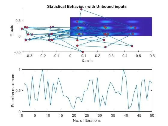
In above plot, it can be observed how the random sampling of the genetic algorithm generates a new optimum value for the function every time the code is run. Although this falls in line with the definition of Genetic Algorithm. Large number of red dots shows values of co-ordinates of x, y varies each time iteration runs.

STUDY 2 : STATISTICAL BEHAVIOUR WITH UPPER AND LOWER BOUNDS

or i = 1:n
    [inputs,fopt(i)] = ga(@stalagmite,2,[],[],[],[],[0;0],[1;1]);
    xopt(i) = inputs(1);
    yopt(i) = inputs(2);
end
study2_time = toc

figure(2)
subplot(2,1,1)
hold on
surfc(xx,yy,-f)
shading interp
xlabel('X-axis')
ylabel('Y-axis')
title('Statistical behaviour with upper and lower bounds')
plot3(xopt,yopt,-fopt,'marker','o','markersize',5,'markerfacecolor','r')
subplot(2,1,2)
plot(-fopt)
xlabel('No. of Iterations')
ylabel('Function maximum')

PLOT FOR STATISTICAL BEHAVIOUR WITH UPPER AND LOWER BOUNDS

The above results show the convergence of x and y values. The number of red dots are less compared to previous plot. This is the result of providing upper and lower bounds to the function.

STUDY 3 : STATISTICAL BEHAVIOUR WITH INCREASING ITERATIONS OF GENERAL ALGORITHM

for i = 1:n
    [inputs,fopt(i)] = ga(@stalagmite,2,[],[],[],[],[0;0],[1;1],[],[],options);
    xopt(i) = inputs(1);
    yopt(i) = inputs(2);
end
study3_time = toc

figure(3)
subplot(2,1,1)
hold on
surfc(xx,yy,-f)
shading interp
xlabel('X-axis')
ylabel('Y-axis')
title('Statistical Behaviour with increasing iterations')
plot3(xopt,yopt,-fopt,'marker','o','markersize',5,'markerfacecolor','r')
subplot(2,1,2)
plot(-fopt)
xlabel('No. of Iterations')
ylabel('Function maximum')

PLOT FOR STATISTICAL BEHAVIOUR WITH INCREASING ITERATIONS OF GENERAL ALGORITHM

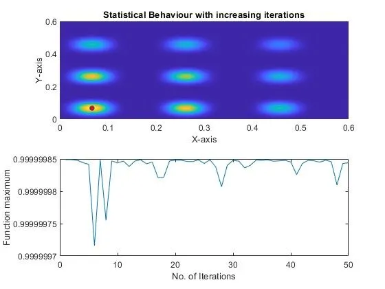
In this study, the number of iterations is increased to 300 to converge and find the global maxima of the function. Here we can see that there is only one red dot on the stalagmite function and that is the required global maxima point.

FINAL PLOT

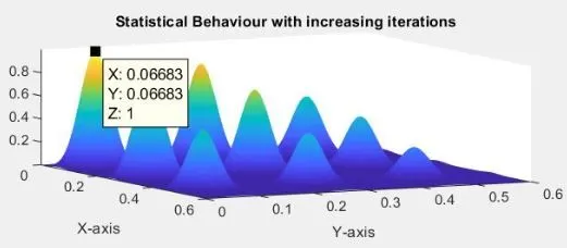
On rotating the plot, we can clearly see the stalagmite function along with the global maxima value as x = 0.06683 and y = 0.06683.