clear all
close all
clc
%inputs
x =linspace(0,0.6,150);
y =linspace(0,0.6,150);
num_spaces=50;
%creating 2D array
[xx yy ] =meshgrid(x,y);
%Evaluating a stalagmite function
for i =1:length(xx)
for j=1:length(yy)
input_vector(1)=xx(i,j);
input_vector(2)=yy(i,j);
f(i,j) = stalagmite_code(input_vector);
end
end
%study 1
tic
for i=1:num_spaces
[results,fopt(i)]=ga(@stalagmite_code,2);
xopt(i)=results(1);
yopt(i)=results(2);
end
study_time=toc
figure(1)
subplot(2,1,1)
surf(x,y,-f)
shading interp
hold on
plot3(xopt,yopt,-fopt,'Marker','o')
subplot(2,1,2)
plot(-fopt)
xlabel('interations')
ylabel('function maximum')
%study 2
tic
for i=1:num_spaces
[results,fopt(i)]= ga( @stalagmite_code,2,[],[],[],[],[0;0],[0.6;0.6]);
xopt(i)=results(1);
yopt(i)=results(2);
end
study_time2=toc
figure(2)
subplot(2,1,1)
surf(x,y,-f)
shading interp
hold on
plot3(xopt,yopt,-fopt,'Marker','o')
subplot(2,1,2)
plot(-fopt)
xlabel('interations')
ylabel('function maximum')
%study 3 population
tic
options=optimoptions('ga');
options=optimoptions(options,'PopulationSize',250);
for i=1:num_spaces
[results,fopt(i)]=ga(@stalagmite_code,2,[],[],[],[],[0;0],[0.6;0.6],[],[],options);
xopt(i)=results(1);
yopt(i)=results(2);
end
study_time3=toc
figure(3)
subplot(2,1,1)
surf(x,y,-f)
shading interp
hold on
plot3(xopt,yopt,-fopt,'Marker','o')
subplot(2,1,2)
plot(-fopt)
xlabel('interations')
ylabel('function maximum')
Stalagmite function code
function A= stalagmite_code(input_vector)
x=input_vector(1);
y=input_vector(2);
f1=(sin(5.1*pi*x+0.5))^6;
f2=exp(-4*log(2)*((x-0.066).^2)/0.64);
f3=(sin(5.1*pi*y+0.5))^6;
f4=exp(-4*log(2)*((y-0.066).^2)/0.64);
A =-(f1*f2*f3*f4);
end
AIM: To write a matlab code of genetic algorithm and calculate the global maxima of stalagmite.
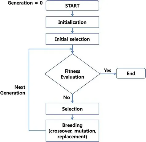
THEORY:Genetic Algorithm are often applied to solve global optimization problems.
As a general rule of the thumb genetic algorithm might be useful in in problem domains that have complex fitness landscape
as mixing i.e , mutation in combination with crossover, is designed to move population away fom local optima that a traditional hill. mutation alone can provide erodicity of the overall genetic algorithm process
The stalagmite function is defined below:
Syntax for genetic algorithm-
x = ga(fun,nvars,A,b,[],[],lb,ub,nonlcon,IntCon,options)
Explaintion of genetic algorithm code
clear all
close all
clc
%inputs
x =linspace(0,0.6,150);
y =linspace(0,0.6,150);
num_spaces=50;
First we initialise the values of x and y taking 150 values between the interval 0 and 0.6
We consider no of iterations num_spaces=50.
%creating 2D array
[xx yy ] =meshgrid(x,y);
%Evaluating a stalagmite function
for i =1:length(xx)
for j=1:length(yy)
input_vector(1)=xx(i,j);
input_vector(2)=yy(i,j);
f(i,j) = stalagmite_code(input_vector);
end
end
Since we need to plot a 3D surface plot we take the 2d array of x and y using meshgrid command and store them in input_vector array ,so that it can be used as an argument to call the function stalagmite
we create another fuction file for the stalagmite function. here we take the ouput as -f since ga only minimises a given function.so if -f is considered it automatically gives us the maxima.
Stalagmite function code
function A= stalagmite_code(input_vector)
x=input_vector(1);
y=input_vector(2);
f1=(sin(5.1*pi*x+0.5))^6;
f2=exp(-4*log(2)*((x-0.066).^2)/0.64);
f3=(sin(5.1*pi*y+0.5))^6;
f4=exp(-4*log(2)*((y-0.066).^2)/0.64);
A =-(f1*f2*f3*f4);
end
now let us make our first study-
we take no of iterations = num_spaces and we use the genetic algorithm function to caluclate the maxima of the function. we store the outputs into results which contain maximas and fopt which contain the value at which the maxima is obtained.
Here the ga is initiated with random population.
%study 1
tic
for i=1:num_spaces
[results,fopt(i)]=ga(@stalagmite_code,2);
xopt(i)=results(1);
yopt(i)=results(2);
end
study_time=toc
figure(1)
subplot(2,1,1)
surf(x,y,-f)
shading interp
hold on
plot3(xopt,yopt,-fopt,'Marker','o')
subplot(2,1,2)
plot(-fopt)
xlabel('interations')
ylabel('function maximum')
store the results into xopt, yopt.now we need to plot the surface of x,y,-f to get the 3D plot.
We use the plot3 command to make a plot of xopt,yopt and -fopt to plot the optimum maximas
forther study 2 as the study1 goes
after that study3 populatin as that code in mention above