Week 5 - Genetic Algorithm

Genetic Algorithm

The genetic algorithm is a method for solving both constrained and unconstrained optimization problems that is based on natural selection, the process that drives biological evolution. The genetic algorithm repeatedly modifies a population of individual solutions. At each step, the genetic algorithm selects individuals at random from the current population to be parents and uses them to produce the children for the next generation. Over successive generations, the population "evolves" toward an optimal solution. You can apply the genetic algorithm to solve a variety of optimization problems that are not well suited for standard optimization algorithms, including problems in which the objective function is discontinuous, nondifferentiable, stochastic, or highly nonlinear. The genetic algorithm can address problems of mixed integer programming, where some components are restricted to be integer-valued.

Generates a population of points at each iteration. The best point in the population approaches an optimal solution. Selects the next population by computation which uses random number generators.

Stalagmite Function

The relation of stalagmite function for global minima is given as;

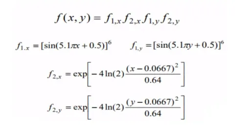
From the above equations, we can create the function of stalagmite.

But, with the above mentioned formula, we can find the global minima. To find global maxima there is a small spin to it.

function [f] = stalagmite(input_vector)
% input_vector(1) = x;
% input_vector(2) = y;
fx = (sin(5.1*pi*input_vector(1)+0.5))^6;
fy = (sin(5.1*pi*input_vector(2)+0.5))^6;
fxx = exp(-4*log(2)*((input_vector(1)-0.0667)^2)/0.64);
fyy = exp(-4*log(2)*((input_vector(2)-0.0667)^2)/0.64);
f = -(fx*fy*fxx*fyy);
end

Main Program :-

%Optimise the stalagmite function
clear all
close all
clc

% 1) input for search space

x = linspace(0,0.6,150);
y = linspace(0,0.6,150);
num_case = 50;

% 2) Use of meshgrid command

[xx,yy] = meshgrid(x,y);

% 3) Evaluating objective function by using nested for loop

for i=1:length(xx)
    for j=1:length(yy)
        input_vector(1)= xx(i,j);
        input_vector(2)= yy(i,j);
        f(i,j) = stalagmite1(input_vector);
    end
end
surfc(x,y,-f)
shading interp

% 1st case study
tic
for i=1:num_case
    [inputs,fopt(i)] = ga(@stalagmite,2);

    xopt(i) = inputs(1);
    yopt(i) = inputs(2);

end

fopt = -fopt
time_study1 = toc

figure(1)
subplot(2,1,1)
hold on
surfc(x,y,-f)
shading interp
plot3(xopt,yopt,fopt,'Marker','o','MarkerSize',5,'MarkerFaceColor','r')
title('bounded inputs')
figure(1)
subplot(2,1,2)
plot(fopt)
xlabel('Iteration')
ylabel('Function maximum')

% 2nd case study
tic
for i=1:num_case
    [inputs2,fopt2(i)] = ga(@stalagmite,2,[],[],[],[],[0,0],[0.6,0.6]);

    xopt2(i) = inputs2(1);
    yopt2(i) = inputs2(2);

end

fopt2 = -fopt2
time_study2 = toc

figure(2)
subplot(2,1,1)
hold on
surfc(x,y,-f)
shading interp
plot3(xopt2,yopt2,fopt2,'Marker','o','MarkerSize',5,'MarkerFaceColor','r')
title('bounded inputs')
figure(2)
subplot(2,1,2)
plot(fopt2)
xlabel('Iteration')
ylabel('Function maximum')

% 3rd case study
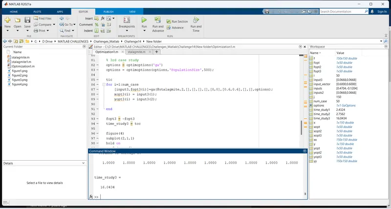
options = optimoptions('ga')
options = optimoptions(options,'PopulationSize',500);

tic
for i=1:num_case
    [input3,fopt3(i)]=ga(@stalagmite,2,[],[],[],[],[0,0],[0.6,0.6],[],[],options);
    xopt3(i) = input3(1);
    yopt3(i) = input3(2);

end

fopt3 = -fopt3
time_study3 = toc

figure(3)
subplot(2,1,1)
hold on
surfc(x,y,-f)
shading interp
plot3(xopt3,yopt3,fopt3,'Marker','o','MarkerSize',5,'MarkerFaceColor','r')
title('bounded inputs')
figure(3)
subplot(2,1,2)
plot(fopt3)
xlabel('Iteration')
ylabel('Function maximum')

Stopping Criteria

It is known that iterative solutions to problems improve initially but deteriorate after some point. This highlights the importance of knowing when it is time to stop. It will not necessarily deteriorate, sometimes the result will remain the same and the iteration goes on and on. In the termination condition of a Genetic Algorithm, it has been observed that initially, the GA progresses very fast with better solutions coming in every few iterations, but this tends to saturate in the later stages where the improvements are very small. We usually want a termination condition such that our solution is close to the optimal, at the end of the run.

Usually, we keep one of the following termination conditions −

1. When there has been no improvement in the population for X iterations.
2. When we reach an absolute number of generations.
3. When the objective function value has reached a certain pre-defined value.

Stopping Condition for Genetic Algorithm

The genetic algorithm uses the following options to determine when to stop. See the default values for each option by running opts = optimoptions('ga').

1. MaxGenerations — The algorithm stops when the number of generations reaches MaxGenerations.
2. MaxTime — The algorithm stops after running for an amount of time in seconds equal to MaxTime.
3. FitnessLimit — The algorithm stops when the value of the fitness function for the best point in the current population is less than or equal to FitnessLimit.
4. MaxStallGenerations — The algorithm stops when the average relative change in the fitness function value over MaxStallGenerations is less than Function tolerance.
5. MaxStallTime — The algorithm stops if there is no improvement in the objective function during an interval of time in seconds equal to MaxStallTime.
6. FunctionTolerance — The algorithm runs until the average relative change in the fitness function value over MaxStallGenerations is less than Function tolerance.
7. ConstraintTolerance — The ConstraintTolerance is not used as stopping criterion. It is used to determine the feasibility with respect to nonlinear constraints. Also, max(sqrt(eps),ConstraintTolerance) determines feasibility with respect to linear constraints.

The algorithm stops as soon as any one of these conditions is met.

Significance of running multiple iterations

Algorithms consist of steps that are carried out one after another. Sometimes an algorithm needs to repeat certain steps until told to stop or until a particular condition has been met. Iteration allows us to simplify our algorithm by stating that we will repeat certain steps until told otherwise.

Its significance in GA can be clearly understood by the fact that, in GA we create as many possiblities we can at first. The iteration helps us to create all of the possiblities in a short span and without repeating the code.

The significance in terms of getting the best result in GA can be found out by increasing the number of studies. The increase in the number of studies gives the result better. In our case, we did 3 studies where in first study we got many points on the graph as maxima. But in second iteration, by giving bound constraints we got selected number of points where the result would lie. But during the next iteration, while optimising we get the exact point of maxima. Sometimes, we may not get the single point, it maybe multiple result from which the maxima will be one. In that case, the maxima can be achieved by doing another study. In this case, 'Global Maxima' was achieved after 3 studies.

Result 1:-

Study 1

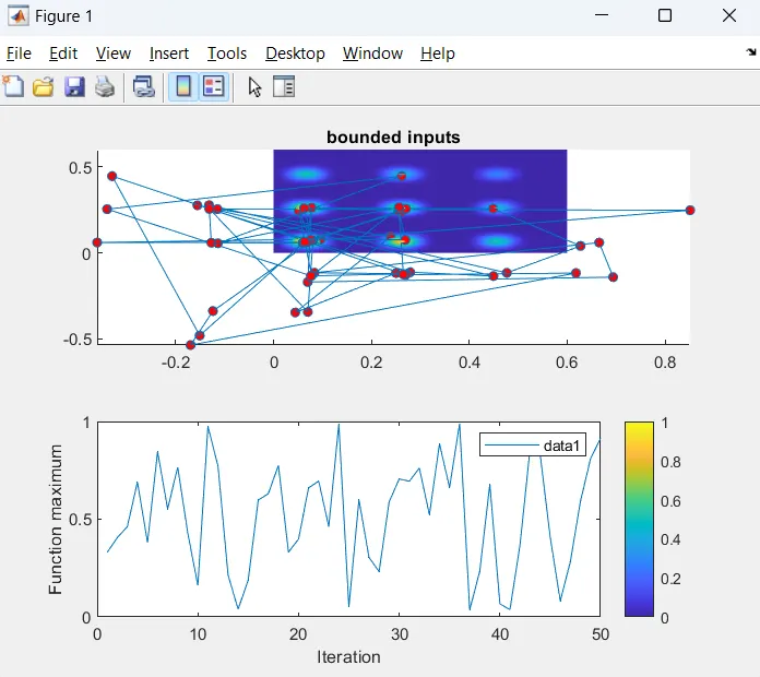
In study 1, we see that the plots has list of scattered point, with no clear Global Maxima Point. This is also called as point where we have result for Population Size. The graph of Iterations against maximu does not clearly indicate the maximum point. The graph can be seen as below;

Study 2

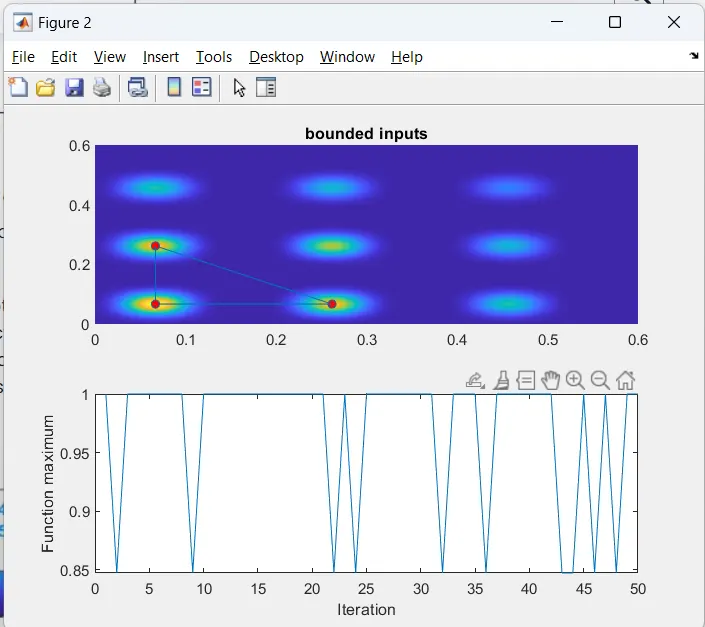
In study 2, we have set the upper and lower limit as well as have set the inequalities to []. What this does is give set of few points where the maxima will be located. The graph of Iterations against Function Maximum will give clear set of point on a graph where maxima will be located. This step is also called as Bound Constraints. The graph can be seen as below;

Study 3

In study 3, we have set the optimisation of 'ga', upper and lower limit, set the inequalities to []. What this does is give exact point where the maxima will be located. The graph of Iterations against Function Maximum will clearly give the point on a graph where maxima will be located. This step is also called as Optimisation. The graph can be seen as below;

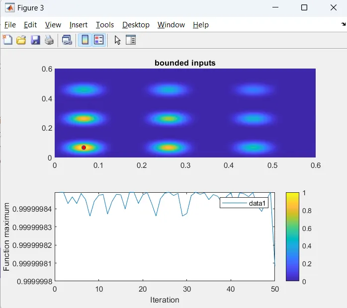
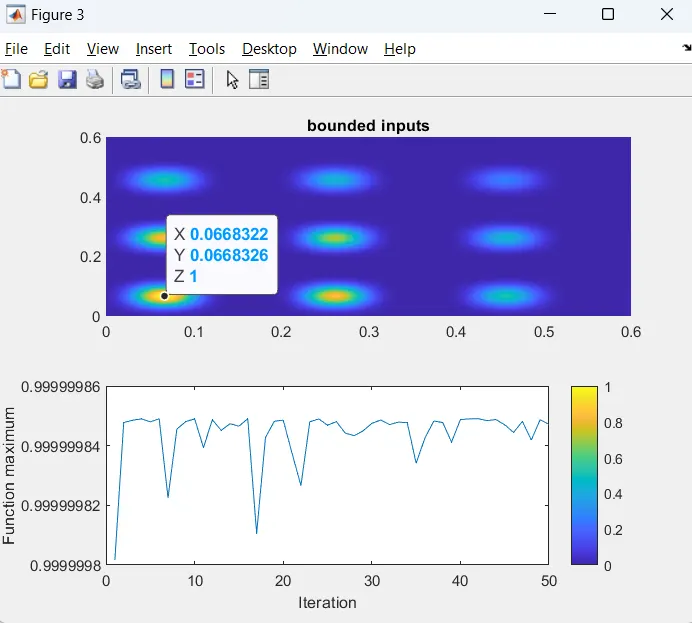
The 'Global Maxima' is 1 located at (0.0668322,0.0668326)