Week 5 - Genetic Algorithm

FUNCTION CODE :

function [f]=stalagmite(input_vector)

x=input_vector(1);

y=input_vector (2);

f1=(sin(5.1*pi*x+0.5))^6;
f2=(sin(5.1*pi*y+0.5))^6;

f3=exp(-4*log(2)*(x-0.0667)^2/0.64);

f4=exp(-4*log(2)*(y-0.0667)^2/0.64);

f=-(f1*f2*f3*f4);
end

MAIN PROGRAM CODE :

% PROGRAM FOR GENETIC ALGORITHM  

clear all
close all
clc
% defining our search space

x=linspace(0,0.6,150);
y=linspace(0,0.6,150);

% creating 2d diamesional mesh

[xx,yy] = meshgrid(x,y);

% evaluting stalagmite function.

for i=1:length(xx)
for j=1:length(yy)
input_vector(1)=xx(i,j);

input_vector(2)=yy(i,j);

f(i,j)=stalagmite(input_vector);

end

end

num_cases=50;

tic

% study 1- stastical behaviour

for i=1:num_cases

[inputs, fopt1(i)] = ga(@stalagmite, 2);
xopt1(i) = inputs(1);

yopt1 (i) = inputs(2);

end

study1_time = toc

figure(1)

subplot(2,1,1)

hold on

surfc(x, y, -f)

shading interp

plot3(xopt1,yopt1,-fopt1,'marker','o','markersize',5,'markerfacecolor','r')
title('unbounded inputs')

subplot(2,1,2)

plot(-fopt1)

xlabel('Interations')

ylabel('function minimum')

tic

%study 2-stastical behaviour - with upper and lower bonds

for i=1:num_cases

[inputs2, fopt2(i)] = ga(@stalagmite,2,[],[],[],[],[0.5:0.5],[1:1]);
xopt2(i) = inputs2(1);

yopt2(i) = inputs2(2);

end

study2_time = toc

figure(2)

subplot(2,1,1)

hold on

surfc(x, y, -f)

shading interp

plot3(xopt2, yopt2, -fopt2,'marker','o','markersize',5,'markerfacecolor','r')

title('unbounded inputs')

subplot(2,1,2)

plot(-fopt2)

xlabel('Interations')
ylabel('function minimum')

% study 3 increasing GA iterations

options = optimoptions('ga');

options = optimoptions(options, 'populationsize', 170)

tic

for i = 1 :num_cases

[inputs3,fopt3(i)] = ga(@stalagmite, 2,[],[],[],[],[0:0],[1:1],[],[],options);
xopt3(i) = inputs3(1);

yopt3(i) = inputs3(2);

end

study3_time = toc

figure(3)

subplot(2,1,1)

hold on

surfc(x, y, -f)

shading interp

plot3(xopt3,yopt3,-fopt3,'marker','o','markersize',5,'markerfacecolor','r')

title('unbounded inputs')
subplot(2,1,2)

plot(-fopt3)

xlabel('Interations')

ylabel('function minimum')

Results :

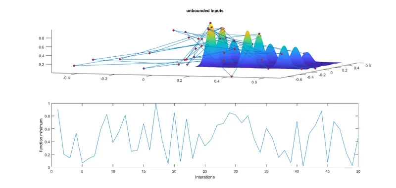
study 1 :

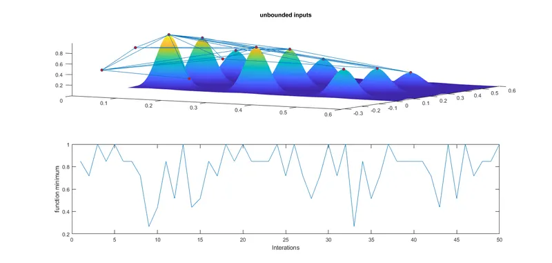
study 2 :

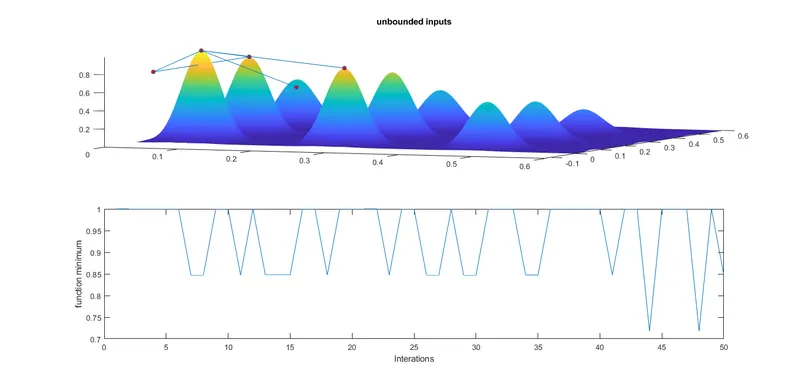
study 3

Explanation :

• First, Linspace command is used to define x and y with 150 elements between zero and 0.6 including the bounds
• Then num_cases is set which will be used as counter for iterations to 50
• Then a 2D grid is made using meshgrid command is created from x and y input to be outputted to xx and yy
• Then for loop is used to solve the genetic algorithm for every element in the 2D mesh grid
• The length of rows and columns (which have equal length) are used as counters
• Then the input vector is declared as ga requires input vector which is each value in the 2D mesh grid
• Then output of stalagmite function is stored in matrix
• Then tic command is used to start a timer
• Then for loop bounded by the number of iterations is formed
• Then ga code is entered for unbounded statistical study which have the following format:[inputs,fopt] = ga(fun,nvars)
• Inputs represent the values of parameters x and y for which the function has the least value (fopt) fun - The function to be optimized
• Then toc command is used to stop the timer and the output is stored in study_time 1
• Then figure 1 is plotted by the following steps:
• First subplot command is used to partition the plot window in order to draw more than one plot in the same windows,two rows and one column are specifiedand then the position of each plot is selected
• Then Hold on command is used to prevent plot from being removed
• Then x, y,and z axis are labeled
• Then shading interp is used to smoothen the function plot and to remove the grid lines
• Then plot 3 command is used to plot a point in 3 dimensions,here it will plot -fopt because we need the maximum value of the function not the minimum
• Then the graph title is selected
• Then -fopt value of the function is plotted on the second plot in the second row
• Then its x and y axis are labeled
• A - Linear inequality constraints: real matrix, if there are none, then[]
• b- Linear inequality constraints: real vector, if there are none, then Aeq - Linear equality constraints: real matrix, if there are none, then[]
• beq - Linear equality constraints: real vector, if there are none, then[]
• lb - Lower bounds, specified as a real vector array ub - Upper bounds, specified as a real vector or array
• The range of the genetic algorithm is Bounded by introducing values for lower and upper bounds and hence the values of global maxima and the values of x and y will be within the defined search space in inputs.
• Then increasing population size study was done which is the same as before but it had different ga code of:[inputs,fopt]-ga(fun,nvars,A,b,Aeq,beq,lb,ub,nonlcon,IntCon,optio inputs, fopt,fun and nvars,A,b,Aeq,beq,lb,ub are the same as Study 1 and Study 2 respectively)
• Then total time is computed
• Then using fprintf command the results are printed in the command windows
• Then the study time is printed
• Then x,y coordinates of the maximum optimum valueare printed
• Then the optimum value of the function (maximum value) is printed which is calculated from the (negative mean) of the all iterations of the output value and the negative sign is used to get the maximum value.
• Then the study time of the whole 3 studies combined is printed.

Syntax for GA :

x-ga(func,nvars,A,B,Aeq,Beq, LB.UB,nonlcon,intcon.options)

func = objective function.

nvars= number of variables.

A & B = subject to inequalities of the form A'x<-B.

Aeq & Beq = subject to linear equalities of the form A*x-B.

LB-lower bond.

UB - upper bond.

nonicon - non linear inequalities

intcon- integrated constraints.

options - helps to add constraints tolerance by increasing population size

Errors :

no errors