Week 5 - Curve fitting

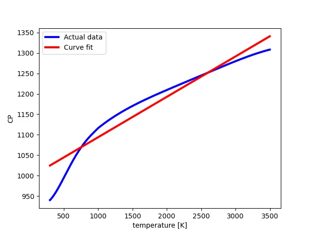
AIM: To fit the curve of the function of linear and cubic polynomial Using python.

Objective:

• To use scipy and numpy modules in the programming.
• To plot the actual curve and the curve fitted of the linear and cubic polynomial.

Introduction:

• Curve fitting is the process of constructing a curve, or mathematical function, that has the best fit to a series of data points, possibly subject to constraints.
• Curve fitting can involve either interpolation, where an exact fit to the data is required, or smoothing, in which a "smooth" function is constructed that approximately fits the data.
• A related topic is regression analysis, which focuses more on questions of statistical inference such as how much uncertainty is present in a curve that is fit to data observed with random errors.
• Fitted curves can be used as an aid for data visualization, to infer values of a function where no data are available, and to summarize the relationships among two or more variables. 
• Extrapolation refers to the use of a fitted curve beyond the range of the observed data, and is subject to a degree of uncertainty since it may reflect the method used to construct the curve as much as it reflects the observed data.
• Scipy is the scientific computing module of Python providing in-built functions on a lot of well-known Mathematical functions. The scipy.optimize package equips us with multiple optimization procedures.

Program-1: To curve fit a linear function.

#Program to curve fit the linear function 
import numpy as np
import matplotlib.pyplot as plt 
from scipy.optimize import curve_fit

#define Curve fir function
def func(t,a,c):
	return a*t + c  #Here linear function is used as curve fit. 

#Defining a function that will read thermodynamic data file present in the same folder of the program.
def read_file(): 
	temperature = [] 
	cp = []
	for line in open('data', 'r'): #Here it opens the data file presented in the same folder and the small r represents read only.
		values = line.split(',') #here the data file is separated by commas and we get two values for each line.
		temperature.append(float(values[0])) #Here the first value is assigned to temperature
		cp.append(float(values[1])) #Here the first value is assigned to  CP.

	return [temperature, cp]

#main program
temperature, cp = read_file() #Calling the Function which reads the value of the Temperature and the cp
popt, pcov = curve_fit(func, temperature, cp) #Here we are dealing with the curve fitting of the function 
fit_cp = func(np.array(temperature), *popt) #Here *popt contains the values for the constants present in our function or equation to be fitted.

#Plotting the curves 
plt.plot(temperature, cp,, linewidth = 3)
plt.plot(temperature, fit_cp,, linewidth = 3)
plt.legend(['Actual data','Curve fit'])
plt.xlabel('temperature [K]')
plt.ylabel('CP')
plt.show()

Output:

Program-2: To curve fit the cubic polynomial.

#Program to curve fit the cubic function 
import numpy as np
import matplotlib.pyplot as plt 
from scipy.optimize import curve_fit

#define Curve fir function
def func(t,a,b,c,d):
	return (a*pow(t,3)) + (b*pow(t,2)) + (c*t) + d  #Here cubic function is used as curve fit. 

#Defining a function that will read thermodynamic data file present in the same folder of the program.
def read_file(): 
	temperature = [] 
	cp = []
	for line in open('data', 'r'): #Here it opens the data file presented in the same folder and the small r represents read only.
		values = line.split(',') #here the data file is separated by commas and we get two values for each line.
		temperature.append(float(values[0])) #Here the first value is assigned to temperature
		cp.append(float(values[1])) #Here the first value is assigned to  CP.

	return [temperature, cp]

#main program
temperature, cp = read_file() #Calling the Function which reads the value of the Temperature and the cp
popt, pcov = curve_fit(func, temperature, cp) #Here we are dealing with the curve fitting of the function 
fit_cp = func(np.array(temperature), *popt) #Here *popt contains the values for the constants present in our function or equation to be fitted.

#Plotting the curves 
plt.plot(temperature, cp,, linewidth = 3)
plt.plot(temperature, fit_cp,, linewidth = 3)
plt.legend(['Actual data','Curve fit'])
plt.xlabel('temperature [K]')
plt.ylabel('CP')
plt.show()

Output:

Questions/Answers:-

1. What does popt and pcov mean?

• Here popt contains the values for the constants present in our function or equation to be fitted.
• Ther pcov contains the estimated co-variance of the values for constants present in popt.
• The Covariance indicates that, how much two random variables vary together. It is similar to variance, but where variance tells you how a single variable varies, co-variance tells you how two variables vary together.

2. What does np.array(temperature) do?

• Here, "np" stands for Numpy module, it is the core library for scientific computing in Python.
• It provides a high-performance multidimensional array object, and tools for working with these arrays.
• A numpy array is a grid of values, all of the same type and is indexed by a tuple of non-negative integers.

3. What does the * in *popt mean?

• The * means that it is reffering to the values present in the popt which are the constants of the function.

4. Write code to fit a linear and cubic polynomial for the Cp data. Explain if your results are good or bad.

• The results for the linear polynomial is not good as the actual data does not obey the linear equation. Also the actual data shows that the plot starts near the origin but the curve fit plot shows there is some variance in the input data.
• The results for the Cubic polynomial is good but not perfect as both the actual plot and the curve fit plot flows the same plot. There is some errors that's why we didn't get the perfect fit in both

 5. What needs to be done in order to make the curve fit perfect?

To make a perfect fit, we need to estimated errors and then we have to eliminate those errors so that the actual data set can be overlap to the curve fit. We can use simple linear regression or the Root mean square (RMS) method to get the perfect fit.