Week 5 - Curve fitting

AIM: Write a program in python to perform curve fitting and determine the fitness of the curve.

OBJECTIVES:

1. To write codes to fit a linear and cubic polynomial for the Cp data.
2. To plot the linear and cubic fit curves along with the raw data points.
3. To measure the fitness characteristics for both the curves.

THEORY:

Curve fitting is constructing a mathematical function which best fits a set of data points.

Fitted curves can be used to help data visualization, to guess values of a function where no data is available, and to summarize the relationships among two or more variables.

Interpolation is a method of estimating values between known data points.

Smoothing is a method of reducing the noise within a data set.

Linear regression (or Linear Curve Fit) is a linear approach to modelling the relationship between a scalar response (or dependent variable) and one or more explanatory variables (or independent variables). Although there might be some curve to your data, a straight line provides a reasonable enough fit to make predictions.

Nonlinear regression is a form of regression analysis in which observational data are modelled by a function which is a nonlinear combination of the model parameters and depends on one or more independent variables. The data are fitted by a method of successive approximations.

Goodness of fit of a statistical model describes how well it fits a set of observations. Measures of goodness of fit typically summarize the discrepancy between observed values and the values expected under the model in question.

To choose the best fit for the curve the following four parameters help us to measure the goodness of fit criteria or how well the equations are representing the given datapoints:

1. The sum of squares due to error or simply sum of square error (SSE),
2. R-Square (R^2),
3. Adjusted R-Square,
4. Root mean squared error (RMSE)

Overfitting is "the production of an analysis that corresponds too closely or exactly to a particular set of data, and may therefore fail to fit additional data or predict future observations reliably".

GOVERNING EQUATION:

Sum of squared error, SSE=∑ni=1[Error(i)2]SSE=∑i=1n[Error(i)2]

Where, Error=|y(i)−valueoff(x)atx(i)|=|y(i)−f(x(i))|Error=|y(i)-valueoff(x)atx(i)|=|y(i)-f(x(i))|

Sum of square of the regression SSR=∑ni=1(f(x(i))−Mean)2SSR=∑i=1n(f(x(i))-Mean)2

Sum of square total, SST=SSR+SSESST=SSR+SSE

From here we can calculate R2=SSRSSTR2=SSRSST

Root Mean Squared Error, RMSE=√(∑ni=1(Y(i)−f(x(i)))2n=)√(SSEn)RMSE=√(∑i=1n(Y(i)-f(x(i)))2n=)√(SSEn)

Where n is the total number of datapoints available

INPUTS: Cp vs Temperature data file

STEPS (WITH EXPLAINATION):

First, we import some modules/libraries necessary for the code viz. math, numpy (as np), mathplotlib.pyplot (as plt) and from scipy.optimize we import curve_fit.

Then we define two function for linear curve fit and cubic curve fit. Later we read input file with the help of open command to open the file and ‘r’ to read the file. Then we extract temperature and cp by using line split (in this case it is separated by comma) to separate the data and return the values into their respective array (one for temperature and second for cp). We make use of append to append the data.

Then we come to our main code/program where we perform curve fit by using ‘curve_fit’ command which takes input as the required function (linear or cubic), temperature, and Cp. 'popt' and 'pcov' are used as output for storing parameters obtained by 'curve_fit'. Another variable named 'fit_cp' is used to stores the new values of Cp calculated by using temperature array. Plots of both raw dataset and predicted dataset are made and compared to find fitness characteristics for both the curves for both linear and cubic polynomial.

To measure the fitness characteristics for both the curves, various parameters such as Sum of Square Error (SSE), Sum of Square of the Regression (SSR), Sum of Square Total (SST), R-Square (R2), Root Mean Square Error (RMSE) are calculated. The plot which has highest R-Square (R2) or closest to 1 is considered to be a good fit.

CODE:

import math
import numpy as np
import matplotlib.pyplot as plt
from scipy.optimize import curve_fit

# Linear Curve fit function
def function_lcf(t, a, b):
return a * t + b

# Cubic Curve fit function
def function_ccf(t, a, b, c, d):
return a * pow(t, 3) + b * pow(t, 2) + c * t + d

# Reading thermodynamic data file
def data():
temperature = []
cp = []
for line in open('data', 'r'):
values = line.split(',')
temperature.append(float(values[0]))
cp.append(float(values[1]))

return [temperature, cp]

# Main Program
temperature, cp = data()

popt, pcov = curve_fit(function_lcf, temperature, cp)
fit_cp_l = function_lcf(np.array(temperature), *popt)
plt.figure(1)
plt.plot(temperature, cp, 'b--')
plt.plot(temperature, fit_cp_l, color='red')
plt.legend(['Actual data', 'Curve fit'])
plt.xlabel('Temperature (K)')
plt.ylabel('Cp')
plt.title('Linear Curve fitting')
plt.show()

popt, pcov = curve_fit(function_ccf, temperature, cp)
fit_cp_c = function_ccf(np.array(temperature), *popt)
plt.figure(2)
plt.plot(temperature, cp, 'b--')
plt.plot(temperature, fit_cp_c, color='red')
plt.legend(['Actual data', 'Curve fit'])
plt.xlabel('Temperature (K)')
plt.ylabel('Cp')
plt.title('Cubic Curve fitting')
plt.show()

#Measuring the fitness characetristics of the curves

s = np.sum(cp)
l = np.size(cp)
m = s / l # Finding mean of Cp data
print('Mean of all cp :', m)
print('') #This will print an empty line (use to give line break)

# For Linear curve fit
linear_sse = 0
linear_ssr = 0
for i in range(l):
linear_error = abs((np.sum((cp[i] - fit_cp_l[i]))))
linear_sse = linear_sse + pow(linear_error, 2)
linear_ssr = linear_ssr + np.sum(pow((fit_cp_l[i] - m), 2))

print('For Linear Curve Fit')
linear_sst = linear_sse + linear_ssr
print('linear_sst :', linear_sst)
linear_R2 = linear_ssr / linear_sst
print('linear_R2 :', linear_R2)
linear_rmse = pow((linear_sse / l), 0.5)
print('linear_RMSE :', linear_rmse)
print('') #This will print an empty line (use to give line break)

# For Cubic curve fit
cubic_sse = 0
cubic_ssr = 0
for j in range(l):
cubic_error = abs(np.sum((cp[i] - fit_cp_c[i])))
cubic_sse = cubic_sse + (pow(cubic_error, 2))
cubic_ssr = cubic_ssr + np.sum(pow((fit_cp_c[i] - m), 2))

print('For Cubic Curve Fit')
cubic_sst = cubic_sse + cubic_ssr
print('cubic_sst :', cubic_sst)
cubic_R2 = cubic_ssr / cubic_sst
print('cubic_R2 :', cubic_R2)
cubic_rmse = pow((cubic_sse / l), 0.5)
print('cubic_RMSE :', cubic_rmse)

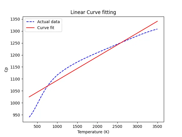
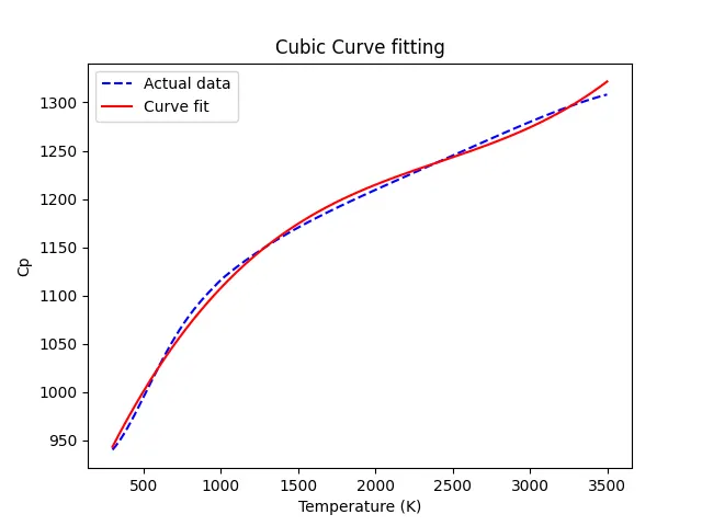
Goodness of fit for linear and cubic curve

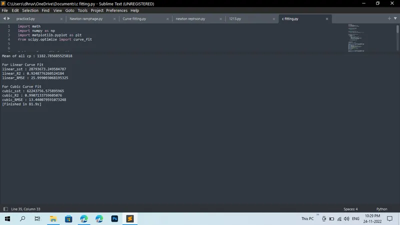
From the outputs we can observe that the values of R-Square (R2) is close to 1 for both linear and cubic curve which indicates the fit is a good fit.

QUESTION-ANSWERS:

Q1. What does popt and pcov mean?

A1. ‘popt’ is an array that stores the values of the coefficients that are being passed in a given function.

‘pcov’ is a two-dimensional array that stores the values of the estimated covariance of ‘popt’ i.e the coefficients.

Q2. What does np.array(temperature) do?

A2. This command converts each value of temperature in the data file into an array using the NumPy module.

Q3. What does the * in *popt mean?

A3. '*' in ‘*popt' indicates and returns each coefficient stored in popt array.

Q4. What needs to be done in order to make the curve fit perfect?

A4. In order to make the curve fit perfect we can increase the order of the polynomial or break the data set into different groups of certain range or both.

CONCLUSION:

Hence, we can conclude that to make the curve fit good R2 should be close to 1. It can be found from the results obtained as for linear curve fit R2 is approximately 0.93 and for the cubic curve fit it is nearly 0.99. So, it can be said that cubic polynomial fits better than linear polynomial. If the order of the polynomial increases, the value of R2 will inch towards 1 and fit will be assumed to be good.