Week 5 - Curve fitting

1. The curve_fit() function will return the optimal values for the objective function. For example, the values of the coefficient. The function will also return a co-variance matrix for the calculated arguments.

2. np.array(temperature) will creates an array of values of temperature values, AS NumPy arrays are stored at one continuous place in memory unlike lists, so processes can access and manipulate them very efficiently.

3. * is a star or Asterisk operator. It is used to pass a variable number of arguments to a function, it is mostly used to pass a non-key argument and variable-length argument list.

4. Code 

#Curve_fit

import numpy as np
import matplotlib.pyplot as plt
from scipy.optimize import curve_fit
#curve fit function

# the below functions solve the polynomial function of specified order and gives the output of coefficients such as a,b,c,d.

#for quadtratic polynomial
def fun(t,a,b,c):
	return a*pow(t,2)+b*t+c
#function for cubic polynomial
def fun_c(t,a,b,c,d):
	return a*pow(t,3)+b*pow(t,2)+c*t+d




#function to read thermodynamic data file
def read_file():
	temp=[] #created a empty array for saving the values of temperature in variable temp
	cp=[] #created a empty array for saving the values of specific heat at constant pressure in the variable cp
	
	for line in open ('data','r'): #for loop is to read the data file line to line
		values=line.split(',') #the values or data in each line will be splited for every comma symbol and saved in the variable values
		temp.append(float(values[0])) #as the first coloum values are temperature values, we save 1st value of array values in temp variable using apped command and float to convert  and save values into float (decimals)
		cp.append(float(values[1])) #and the second coloum values are specific heat at constant pressure values, we save 2nd value of array values in cp variable
	return [temp, cp] #after the read function it returns the values of temperature and specific heat at constant pressure

temp,cp=read_file() # calling the read funciton and the retured values of temp and cp are saved

popt,pcov=curve_fit(fun, temp, cp) #we imported curve fitting command from scipy module, which calculates the polynomial function and returns the optimal values for the mapping function, e.g, the coefficient values. It also returns a covariance matrix for the estimated parameters 
fit_cp=fun(np.array(temp),*popt) #to calulate the fitted value of specific heat at constant pressure we again call the polynomial function of each value of temperature (using numpy module) as t and coefficents as optimal values returned from above syntax and It  is used to pass a variable number of arguments to a function, * used to pass a non-key argument and variable-length argument list. 


popt_3,pcov=curve_fit(fun_c, temp, cp) #similarly for cubic polynomial
fit_cp_3=fun_c(np.array(temp),*popt_3)


plt.plot(temp,cp,color='green',linewidth=1) #here we plot the original curve passing through our given data (temperature Vs specific heat)
plt.plot(temp,fit_cp,color='red',linewidth=1) #plot for quadratic polynomial solved values of specific heat Vs temperature curve

plt.plot(temp,fit_cp_3,color='yellow',linewidth=1)#plot for cubic polynomial solved values of specific heat Vs temperature curve


plt.legend(['actual data','curve fit','cubic curve fit']) #legend to distinguish the curve
plt.xlabel('temperature') 
plt.ylabel('cp')
plt.show()

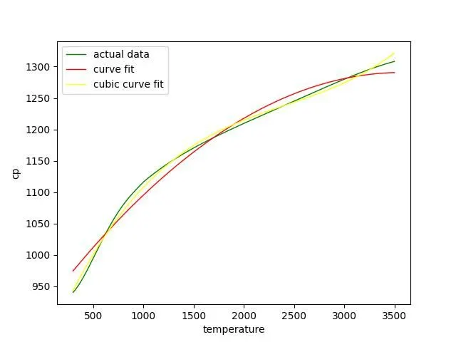
From the output graphs, the results are good because the cubic fit is better to curve fit than the linear one 

5. in order to make the curve fit perfectly, increase the degree of the curve. but might increase the complexity of mathematical calculations

or else divide into the data and solve different polynomial equations for each data set.

6.