Week 5 - Curve fitting

CURVE FITTING

Introduction:

• curve_fit is a process of construction of curve, or mathematical function that has a best fit to series of data points possibly subject to constraints. Curve fitting can involve either interpolations where an exact fit to the data is required.
• In this challenge we will try to fit the linear and cubic polynomial to best fit the curve obtained bt the given data of temperature and specific heat at constant pressure (Cp).
• It is a statistical technique used to drive coefficient values for equations that express the value for one (dependent) variable as a function of another (independent variable)
• It has its engineering application in trend analysis, hypothesis testing (which is used to compare existing mathematical model with measured data.

1.What does popt and pcov mean?

popt is an array with the optimal parameters obtained using a non-linear least squaresfit. pcov is a 2d array with the estimated covariance of the parameters in popt.

2.What does np.array(temperature) do?

A numpy array is a grid of values, all of the same type. Here it is being used to pass the values of temperatue to the function.

3.What does the in popt mean?

The star here means that it is being referenced. Any and all change which could have occure to popt while in a function would be reflected in the original popt.

4.What needs to be done in order to make the curve fit perfect?

A curve fit can almost never be perfect because experimental data will always vary from a perfect equation. However the fit can be made as close as possible by trying different order equations, extrapolation, dividing the data and curve fitting them seperately or on very rare case finding an equation which fits the data perfectly.

Code Explanation

• Required Libraries including numpy, scipy. optimize and matplotlib.pyplot are imported
• Fun1, fun2, fun3, and fun4 are programmed to accept the values of t, a, b, c and d and to return the value after calculating by using them all in cubic and linear equations respectively.
• The thermodynamic values file is read using read function, its value is seperated using split function and stored in two different matrices called temperature and cp.
• popt and pcov values are found out using curve_fit function. Further the calculated values are stored by calling fun function for cubic equations and stored in fit_cp.
• Popt1 and pcov1 values are found out using curve_fit function. Further the calculated values are stored by calling func1 function for Linear equations and stored in fit_cp1.

Code:

import matplotlib.pyplot as plt
import numpy as np
from scipy.optimize import curve_fit

#define the function to read the notepad data file
def read_file():
    temperature = []
    cp = []
    for line in open('data','r'):
        values = line.split(',')
        temperature.append(float(values[0]))
        cp.append(float(values[1]))
    
    return [temperature,cp]

#define the function for curve fittng
def fun1(t,a,b,c,d,e):
    return a*t + b
def fun2(t,a,b,c,d,e):
    return a*t**2 + b*t + c
def fun3(t,a,b,c,d,e):
    return a*t**3 + b*t**2 + c*t + d
def fun4(t,a,b,c,d,e):
    return a*t**4 + b*t**3 + c*t**2 + d*t + e

#for labeling the respective graphs with corresponding fitting function
i = -1
label_fun = [r'$1st$',r'$2nd$',r'$3rd$', r'$4rd$']

#main program
temperature,cp = read_file()
for fun in (fun1,fun2,fun3,fun4):
    popt, pcov = curve_fit(fun, temperature, cp)
    cp_fit_data = fun(np.array(temperature), *popt)
    i = i+1
    print(popt,pcov,cp_fit_data)
    #plotting the real data and the curve fitting data
    plt.plot(temperature, cp_fit_data,color = 'red', linestyle = '-',label = 'curve_fitted with function: f(t)=({})'.format(label_fun[i]))
    plt.plot(temperature,cp, label = 'real plot')
    plt.grid(True)
    plt.xlabel('Temperature (kelvin)')
    plt.ylabel(r'$C_p$')
    plt.title('curve_fitting_practice')
    plt.legend(loc= 'lower center')
    plt.savefig('{}'.format(i))
    plt.show()

Output:

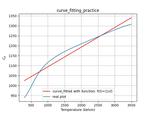
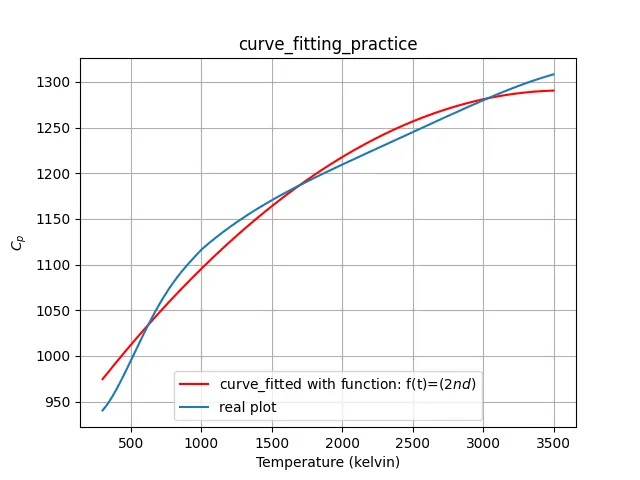
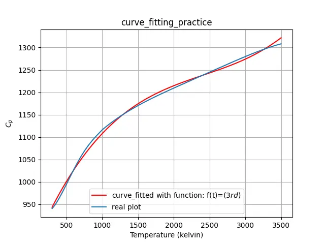
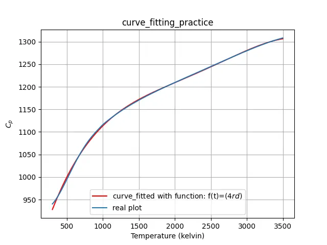
Conclusion:

1. The curve_fit was performed using 4 different fit functions.
2. The curve_fit became more and more accurate as the order of the fit function increased.