Week 5 - Curve fitting

AIM:

Write code to fit a linear and cubic polynomial for the Cp data.

PROCEDURE :

1. popt - it s an array of optimal values for paremeters which and which minimize the sum of sequence of residuals

2. pcov - it is the 2d array which containts the covariance of popt and the diagonals provide the variance of estimated parameter

3. np.array - it converts the python list of temperature to anumpy array

4.

A)For linear polynomial

a. importing math , matplot , numpy and curve_fit functions

b.defining the function of linear polynomial

def func(t,a,b,c,d,e)

c. data file can be move into the same folder of saving python file

d.defining the function reading of thermodynamic data file

e.by using the function of loop to all temperatue and cp lines inthe data file

f. making the progam for curve fitting temperature and cp in the file, as given below,

temperature , cp = read_file()
popt , pcov = curve_fit(func , temperature ,cp)
fit_cp = func(np.array(temperature), *popt)

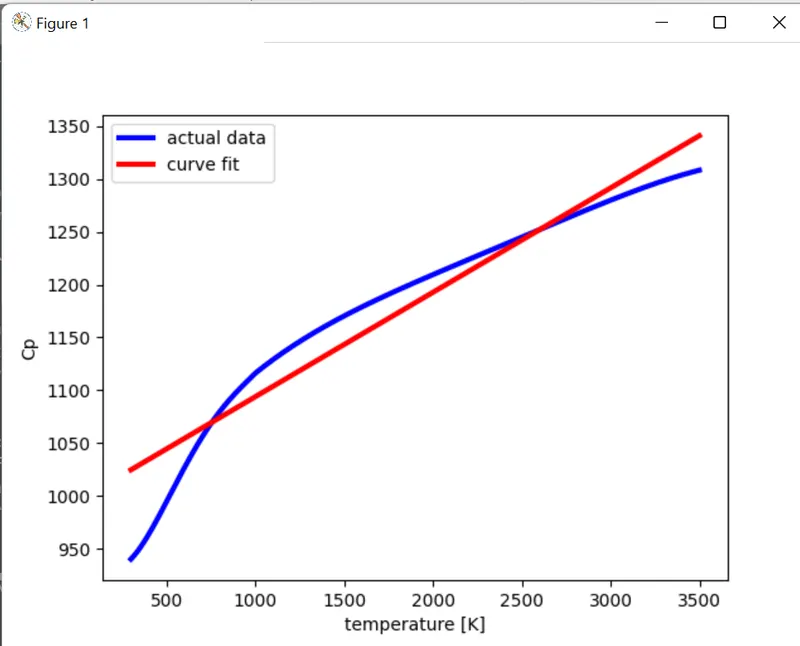
g. making plot for temperature vs cp and temperature vs fit_cp

output plot is ,

B) For cubic polynomial

a.defining the function of linear polynomial

def func(t,a,b,c,d)

b.defining the function reading of thermodynamic data file

c.by using the function of loop to all temperatue and cp lines inthe data file

d. making the progam for curve fitting temperature and cp in the file, as given below,

temperature , cp = read_file()
popt , pcov = curve_fit(func , temperature ,cp)
fit_cp = func(np.array(temperature), *popt)

e. making plot for temperature vs cp and temperature vs fit_cp

output plot is ,

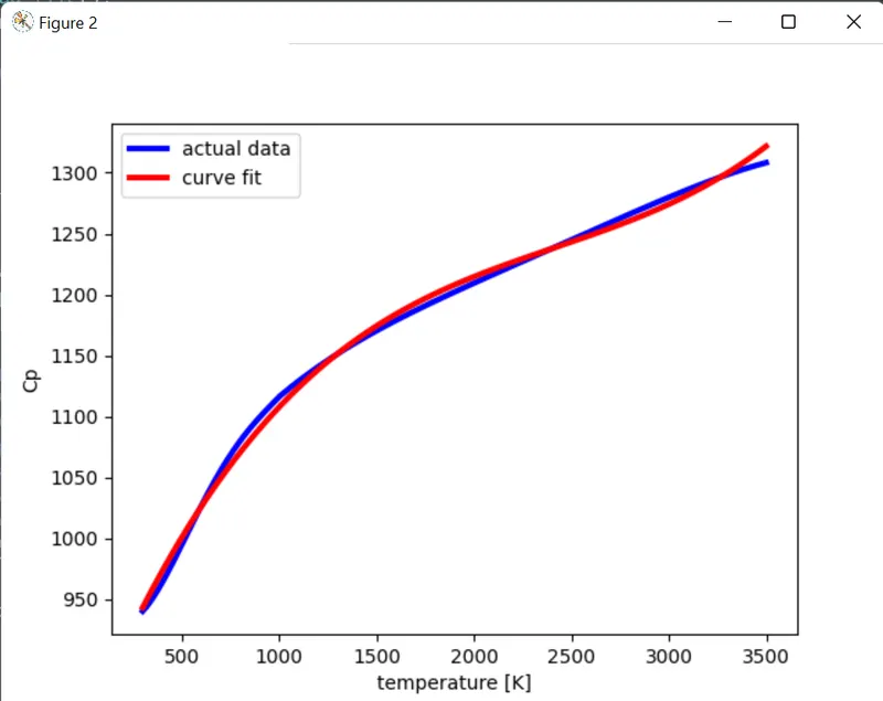
----the cubic fit is better curve_fit than the linear fit ,that can be see from the output plots.

5. - by increase the degree of curve make the best curve fit

- increase the degree of curve in linear , when it is more accurate than cubic polynomial

CONCLUSION :

can be make the coding for polynomial curve_fiting and cubic curve_fiting

import math
import matplotlib.pyplot as plt
import numpy as np
from scipy.optimize import curve_fit

# linear fit function (linear polynomial)
def func(t,a,b,c,d,e):
	return a*t + b

# reading  thermodynamic data file
def read_file():
	temperature = []
	cp = []
	for line in open ('data','r'):
		values = line.split(',')
		temperature.append(float(values[0]))
		cp.append(float(values[1]))

	return [temperature, cp]


# main program
temperature , cp = read_file()
popt , pcov = curve_fit(func , temperature ,cp)
fit_cp = func(np.array(temperature), *popt)

plt.figure(1)
plt.plot(temperature,cp,color="blue",linewidth=3)
plt.plot(temperature,fit_cp,color="red",linewidth=3)
plt.legend(['actual data','curve fit'])
plt.xlabel('temperature [K]')
plt.ylabel('Cp')
plt.show()


# cubic fit function (cubic polynomial)
def func(t,a,b,c,d):
	return a*pow(t,3) + b*pow(t,2) + c*t + d

# reading thermodynamic data file 	
def read_file():
	temperature = []
	cp = []
	for line in open ('data','r'):
		values = line.split(',')
		temperature.append(float(values[0]))
		cp.append(float(values[1]))

	return [temperature, cp]			

# main program
temperature , cp = read_file()
popt, pcov = curve_fit(func , temperature ,cp)
fit_cp = func(np.array(temperature), *popt)

plt.figure(2)
plt.plot(temperature,cp,color="blue",linewidth=3)
plt.plot(temperature,fit_cp,color="red",linewidth=3)
plt.legend(['actual data','curve fit'])
plt.xlabel('temperature [K]')
plt.ylabel('Cp')
plt.show()