Week 5 - Curve fitting

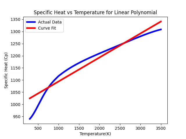
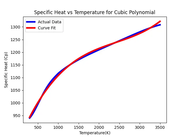
Aim: To write code to fit a linear and cubic polynomial for the Cp data and explain if the results are favorable or not.

Theory:

Curve Fitting is the process of constructing a curve through mathematical function that best fits to a series of data points, possible subject to constraints. Curve fit function returns two items, PCOV and POPT.

PCOV - It contains the covariance matrix for the fit parameters, which indicates the uncertainties and correlations between parameters. This is most useful when the data has uncertainties.

POPT - It is an array that provides an optimal value so that the sum of the squared residuals of the function. In general, the return value 'popt' contains the best fit values of the parameters.

np.array(temperature) - The array object in numpy is called np.array. This function stores the values of temperature as an array and passes it to numpy function.

*popt - The asterisk (*) in *popt is used to store the values of constant parameters (a,b,c) in the array popt.

Code:

import numpy as np
import matplotlib.pyplot as plt
from scipy.optimize import curve_fit

#Reading the given thermodynamic data file
def readfile():
	temperature = []
	cp = [] #specific heat
	for line in open('data','r'):	#reads everyline in 'data'
		values = line.split(',')	#splits line by comma
		temperature.append(float(values[0]))
		cp.append(float(values[1]))
	return [temperature,cp]

#Linear Curve fit definition
def Linear_func(t,a,b):
	x = a*t+b 			#a,b variables and t is temp
	return x

#Code to read file and give output
temperature,cp=readfile()
popt,pcov = curve_fit(Linear_func,temperature,cp)
fit_cp = Linear_func(np.array(temperature),*popt)

#Plotting graph for linear curve fit
plt.figure(1)
plt.plot(temperature,cp,color='blue',linewidth=4)
plt.plot(temperature,fit_cp,color='red',linewidth=4)
plt.title('Specific Heat vs Temperature for Linear Polynomial')
plt.legend(['Actual Data','Curve Fit'])
plt.xlabel('Temperature(K)')
plt.ylabel('Specific Heat (Cp)')
plt.savefig('Linear Polynomial Curve Fit')
plt.show()

#Cubic Curve fit definition
def Linear_func(t,a,b,c,d):
	x = a*t**3+b*t**2+c*t+d 			#a,b,c,d variables and t is temp
	return x

#Code to read file and give output
temperature,cp=readfile()
popt0,pcov0 = curve_fit(Linear_func,temperature,cp)
fit_cp = Linear_func(np.array(temperature),*popt0)

#Plotting graph for linear curve fit
plt.figure(2)
plt.plot(temperature,cp,color='blue',linewidth=4)
plt.plot(temperature,fit_cp,color='red',linewidth=4)
plt.title('Specific Heat vs Temperature for Cubic Polynomial')
plt.legend(['Actual Data','Curve Fit'])
plt.xlabel('Temperature(K)')
plt.ylabel('Specific Heat (Cp)')
plt.savefig('Cubic Polynomial Curve Fit')
plt.show()

Code Explanation:

• import numpy, matplotlib.pylot.
• import curve_fit from scipy.optimize
• Read the given thermodynamic data file in a separate function called readfile()
• Use a "for" loop to read the file, line-by-line.
• Append each value between commas into arrays for temperature and Specific Heat (Cp) respectively.
• Define a linear function (at+b) and return its result.
• Use curve_fit function to calculate the value linear function using temperature and Specific Heat (Cp) from the given data file.
• Using the function again to fit the curve taking temperature and Specific Heat (Cp) values from the array and the values of parameters from *popt. The result is stored in fit_cp.
• Repeat the same steps for cubic polynomial (at^3+bt^2+ct+d).
• We now have the data to create plots for linear and cubic plynomials and can compare the curve fit of the equations.

Conclusion:

The curve fit can never be perfect; experimental value and the ideal curve-fit value will always vary. However, the proximity to the required curve can be improved. This can be seen by the code and graph shown. As the order of the equations increase, the value gets closer to the ideal value. There are other methods like dividing the data and curve fitting them separately or extrapolation.

By the above graphs, we can conclude that with the increase in the order of the polynomial, the value of actual data comes closer to the ideal curve fit.