Week 5 - Curve fitting

Aim:

Scripting the code to provide the linear and cubic polynomial for the given data.

popt:

An array of optimal values for the parameters which minimizes the sum of squares of residuals.

pcov:

The returned parameter covariance matrix pcov is based on scaling sigma by a constant factor.

np.array:

To make a numpy array, you can just use the np. array() function. All you need to do is pass a list to it, and optionally, you can also specify the data type of the data.

* in *popt mean

Here * is reference to popt / the values stored in the array popt.

Curve Fitting:

Curve fitting is one of the most powerful and most widely used analysis tools in Origin. Curve fitting examines the relationship between one or more predictors (independent variables) and a response variable (dependent variable), with the goal of defining a "best fit" model of the relationship.

Non linear curve:

Non-linear curve fitting makes it possible to converge a model function dependent on an independent variable and several parameters toward a given data set. This analysis object is primarily used for determining model parameters so that the selected model is adapted to the data in the best way possible.

scipy optimize:

This provides the flexibility and control to define the form of the curve, where an optimization process is used to find the specific optimal parameters of the function. ... The SciPy Python library provides an API to fit a curve to a dataset.

Float option:

Here the Python float() method converts a number stored in a string or integer into a floating point number, or a number with a decimal point.

Program:

import numpy as np
import matplotlib.pyplot as plt
from scipy.optimize import curve_fit

#cubic polynomial
def fun2(t,a,b,c,d):
	return a*pow(t,3)+b*t*t+c*t+d

#linear polynomial
def fun3(t,a,b,c):
	return a*t+b

#reading thermodynamics data file
def read_file():
	temperature = []
	cp = []
	for line in open('data','r'):
		value = line.split(',')
		temperature.append(float(value[0]))
		cp.append(float(value[1]))
	return[temperature,cp]

temperature,cp = read_file()

#cubic polynomial
popt2,pcov2 = curve_fit(fun2,temperature,cp)
fit_cp2 = fun2(np.array(temperature),*popt2)
plt.plot(temperature,cp,color='green',linewidth=3)
plt.plot(temperature,fit_cp2,color='blue',linewidth=3)
plt.legend(['actual data','curve_fit'])
plt.xlabel('temp[k]')
plt.ylabel('cp')
plt.title('cubic')
plt.show()

#linear polynomial
popt3,pcov3 = curve_fit(fun3,temperature,cp)
fit_cp3 = fun3(np.array(temperature),*popt3)
plt.plot(temperature,cp,color='green',linewidth=3)
plt.plot(temperature,fit_cp3,color='orange',linewidth=3)
plt.legend(['actual data','curve_fit'])
plt.xlabel('temp[k]')
plt.ylabel('cp')
plt.title('linear')
plt.show()

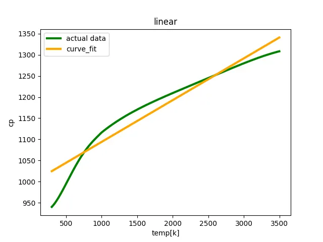
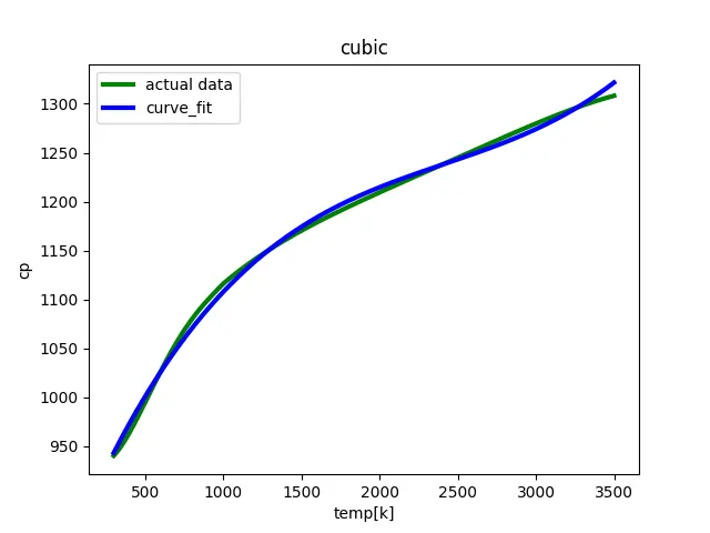
Graph accorded depends on the program:

Linear polynomial:

Cubic polynomial:

In order to make the curve fit perfect:

The curve fit cannot be made perfect because it is experimental data and varies from the perfect equation. However the curve fit can be made close perfect by trying the different order equation.

Result:

From the graph it can be seen that the curve fits better in cubic polynomial that the linear polynomial.