Week 5 - Curve fitting

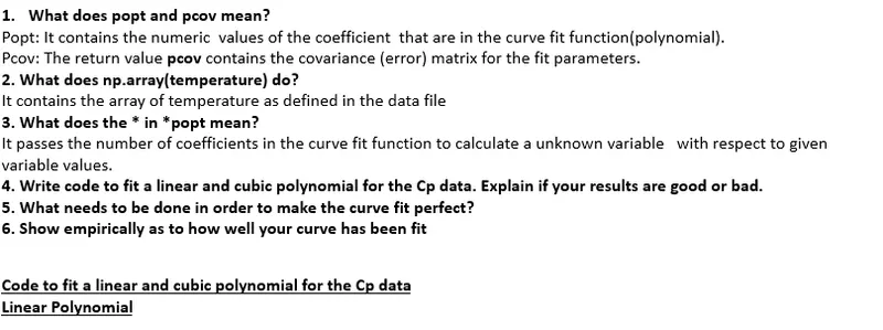
Steps Followed:

1.Import Modules in sublime text

Import numpy as np
import matplotlib.pyplot as plt
from scipy.optimize import curve_fit

2. Call a function

def func(t,a,b): # calling a function
return a*t+b

3. Call a function that returns temperature and cp value contained in the data file.

def read_file():
temperature=[] # temperature array
cp=[] # specific heat array
for line in open('data','r'): # loop for reading a data file
values=line.split(',') # splitting the values in data file
temperature.append(float(values[0])) # appending the temperature array
cp.append(float(values[1])) # appending the specific heat array
return[temperature,cp]

4. Write a curve fit function which solves cp for given temperature

temperature,cp=read_file()
popt,pcov=curve_fit(func,temperature,cp) # Curve fit function
fit_cp=func(np.array(temperature),*popt) # Curve fitting the cp with respect to temperature

5. Plot the results

import numpy as np
import matplotlib.pyplot as plt
from scipy.optimize import curve_fit
# Curve fit function
def func(t,a,b): # calling  a function
	return a*t+b

# Reading thermodynamic data file
def read_file():
	temperature=[] # temperature array
	cp=[] # specific heat array
	for line in open('data','r'): # loop for reading a data file 
		values=line.split(',') # splitting the values in data file 
		temperature.append(float(values[0])) # appending the temperature array
		cp.append(float(values[1])) # appending the specific heat array
	return[temperature,cp]
# Main Program
temperature,cp=read_file()
popt,pcov=curve_fit(func,temperature,cp) # Curve fit function 
fit_cp=func(np.array(temperature),*popt) # Curve fitting the cp with respect to temperature  
# plotting
plt.plot(temperature,cp,color="blue",linewidth=1) 
plt.plot(temperature,fit_cp,color="red",linewidth=1)
plt.legend(['Actual data','Curve Fit'])
plt.xlabel('Temperature [K]')
plt.ylabel('Cp')
plt.grid('on')
plt.show()

Cubic Polynomial

import numpy as np
import matplotlib.pyplot as plt
from scipy.optimize import curve_fit
# Curve fit function
def func(t,a,b,c,d): # calling  a function
	return a*pow(t,3)+b*pow(t,2)+c*t+d

# Reading thermodynamic data file
def read_file():
	temperature=[] # temperature array
	cp=[] # specific heat array
	for line in open('data','r'): # loop for reading a data file 
		values=line.split(',') # splitting the values in data file 
		temperature.append(float(values[0])) # appending the temperature array
		cp.append(float(values[1])) # appending the specific heat array
	return[temperature,cp]
# Main Program
temperature,cp=read_file()
popt,pcov=curve_fit(func,temperature,cp) # Curve fit function 
fit_cp=func(np.array(temperature),*popt) # Curve fitting the cp with respect to temperature  
# plotting
plt.plot(temperature,cp,color="blue",linewidth=1) 
plt.plot(temperature,fit_cp,color="red",linewidth=1)
plt.legend(['Actual data','Curve Fit'])
plt.xlabel('Temperature [K]')
plt.ylabel('Cp')
plt.grid('on')
plt.show()

..

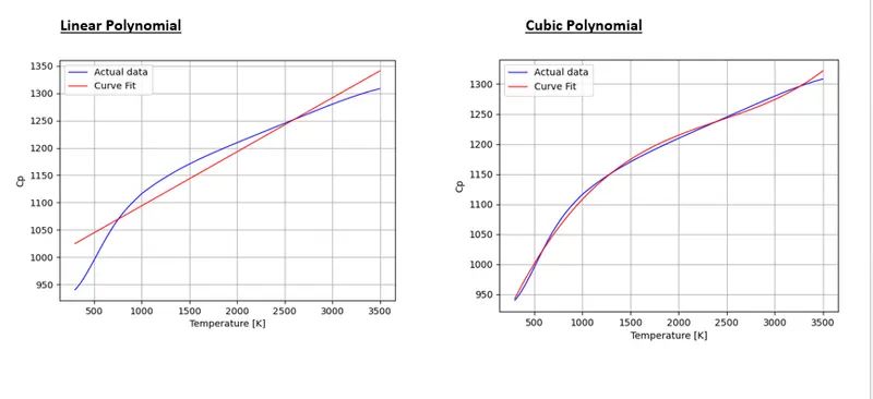
As it can be seen from the above data that the cubic polynomial has better curve fit as compared to linear polynomial. In order to make the curve fit perfect,higher order polynomial curve fit has to be performed for better results.

R Square method is used to check for the goodness of Curve fit

For Linear Polynomial

import numpy as np
import matplotlib.pyplot as plt
from scipy.optimize import curve_fit
# Curve fit function
def func(t,a,b): # calling  a function
	return a*t+b
# Reading thermodynamic data file
def read_file():
	temperature=[] # temperature array
	cp=[] # specific heat array
	for line in open('data','r'): # loop for reading a data file 
		values=line.split(',') # splitting the values in data file 
		temperature.append(float(values[0])) # appending the temperature array
		cp.append(float(values[1])) # appending the specific heat array
	return[temperature,cp]
# Main Program
temperature,cp=read_file()
popt,pcov=curve_fit(func,temperature,cp) # Curve fit function 
fit_cp=func(np.array(temperature),*popt) # Curve fitting the cp with respect to temperature  
# plotting
plt.plot(temperature,cp,color="blue",linewidth=1) 
plt.plot(temperature,fit_cp,color="red",linewidth=1)
plt.legend(['Actual data','Curve Fit'])
plt.xlabel('Temperature [K]')
plt.ylabel('Cp')
plt.grid('on')
plt.show()


# To check the goodness of fit Using R Square Method 
# Sum of squares of errors (SSE)
SSE=np.sum(pow((np.array(np.array(cp)-np.array(fit_cp))),2))
# Sum of squares of regression (SSR)
SSR=np.sum(pow((np.array(np.array(fit_cp)-np.mean(cp))),2))
# Total sum of squares 
SST=SSR+SSE
# R-Square value  
R2=SSR/SST
print('The R square value is ',R2)

For Cubic Polynomial

import numpy as np
import matplotlib.pyplot as plt
from scipy.optimize import curve_fit
# Curve fit function
def func(t,a,b,c,d): # calling  a function
	return a*pow(t,3)+b*pow(t,2)+c*t+d

# Reading thermodynamic data file
def read_file():
	temperature=[] # temperature array
	cp=[] # specific heat array
	for line in open('data','r'): # loop for reading a data file 
		values=line.split(',') # splitting the values in data file 
		temperature.append(float(values[0])) # appending the temperature array
		cp.append(float(values[1])) # appending the specific heat array
	return[temperature,cp]
# Main Program
temperature,cp=read_file()
popt,pcov=curve_fit(func,temperature,cp) # Curve fit function 
fit_cp=func(np.array(temperature),*popt) # Curve fitting the cp with respect to temperature  
# plotting
plt.plot(temperature,cp,color="blue",linewidth=1) 
plt.plot(temperature,fit_cp,color="red",linewidth=1)
plt.legend(['Actual data','Curve Fit'])
plt.xlabel('Temperature [K]')
plt.ylabel('Cp')
plt.grid('on')
plt.show()


# To check the goodness of fit Using R Square Method 
# Sum of squares of errors (SSE)
SSE=np.sum(pow((np.array(np.array(cp)-np.array(fit_cp))),2))
# Sum of squares of regression (SSR)
SSR=np.sum(pow((np.array(np.array(fit_cp)-np.mean(cp))),2))
# Total sum of squares 
SST=SSR+SSE
# R-Square value  
R2=SSR/SST
print('The R square value is ',R2)

Conclusion:

As it can been seen that Goodness of fit has been performed using the R Square method,it can be clearly seen that the R square value for cubic polynomial is very close to 1 compared to linear polynomial. that shows higher the order of the polynomial, higher will be the accuracy.