Week 5 - Curve fitting

1. What does popt and pcov mean?

Sol: popt represents the matrix that stores and extracts the coefficients for the fitting functions according to the general equations defined.

whereas pcov represents the square matrix which stores the estimated values of covariance of the coefficients of the above. The diagonal elements of this square matrix also represent the variance of that coefficients.

2. What does np. array(temperature) do?

Sol: np.array command converts each value of the temperature in the data file into the form of an array using the numpy module.

3. What does the * in *popt mean?

Sol: popt defines and returns each coefficient stored in popt array.

4 & 6. Write code to fit a linear and cubic polynomial for the Cp data. Explain if your results are good or bad. & Show empirically how well your curve has been fit.

Sol:

#Curve Fitting Challenge

#Importing all the Libraries

import math
import matplotlib.pyplot as plt 
import numpy as np 
from scipy.optimize import curve_fit

#Defining a function for solving in linear polynomial 

def f_order1(t,a,b):

	a*t + b
	return a*t + b

#Defining a function for solving in cubic polynomial 

def f_order3(t,a,b,c,d):

	a*pow(t,3) + b*pow(t,2) + c*t + d
	return a*pow(t,3) + b*pow(t,2) + c*t + d

#reading data from the file, named 'data'

def read_file():
	
	temperature = []
	cp = []
	for line in open ('data','r'): # reading each line of file
		line=line.split(',')
		temperature.append(float(line[0])) # storing the values of temperature in temperature array
		cp.append(float(line[1]))          # storing the values of cp in array cp
		
	return [temperature, cp]

# Optimizing the curve for linear polynomial

temperature, cp = read_file()
popt_1, pcov_1 = curve_fit(f_order1, temperature, cp)
new_cp_1 = f_order1(np.array(temperature), *popt_1)

#Calculating goodness of linear fit

#SSE
sse = 0
for i in range(0,np.size(cp)):
	sse = sse + pow(cp[i]-new_cp_1[i],2)

print('For linear polynomial fit,')

#R_square 
mean =np.sum(cp)/np.size(cp)
ssr=0
for i in range(0,np.size(cp)):
	ssr = ssr + pow(new_cp_1[i] - mean,2)

sst = ssr + sse 
R_square = ssr/sst
print('R_square = ',R_square)

#RMSE
rmse=pow(sse/np.size(cp),0.5)
print('RMSE = ',rmse)

# Optimizing the curve for cubic polynomial

temperature, cp = read_file()
popt_3, pcov_3 = curve_fit(f_order3, temperature, cp)
new_cp_3 = f_order3(np.array(temperature), *popt_3)

#Calculating goodness of cubic polynomial fit

#SSE
sse = 0
for i in range(0,np.size(cp)):
	sse = sse + pow(cp[i]-new_cp_3[i],2)

print('For cubic polynomial fit,')

#R_square 
mean =np.sum(cp)/np.size(cp)
ssr=0
for i in range(0,np.size(cp)):
	ssr = ssr + pow(new_cp_3[i] - mean,2)

sst = ssr + sse 
R_square = ssr/sst
print('R_square = ',R_square)

#RMSE
rmse=pow(sse/np.size(cp),0.5)
print('RMSE = ',rmse)

#Plotting for linear polynomial curve fit

plt.figure(1)
plt.plot(temperature, cp, linewidth=3, color='blue')
plt.plot(temperature, new_cp_1, linewidth=3, color='red')
plt.legend(['actual data', 'curve fit'])
plt.xlabel('Temperature[K]')
plt.ylabel('cp')
plt.grid()
plt.title('Linear polynomial curve fit')
plt.savefig('Linear polynomial curve fit.png')
plt.show()

#Plotting for cubic polynomial curve fit

plt.figure(2)
plt.plot(temperature, cp, linewidth=3, color='blue')
plt.plot(temperature, new_cp_3, linewidth=3, color='red')
plt.legend(['actual data', 'curve fit'])
plt.xlabel('Temperature[K]')
plt.ylabel('cp')
plt.grid()
plt.title('Cubic polynomial curve fit')
plt.savefig('Cubic polynomial curve fit.png')
plt.show()

Output:

Explanation for the Code Result:

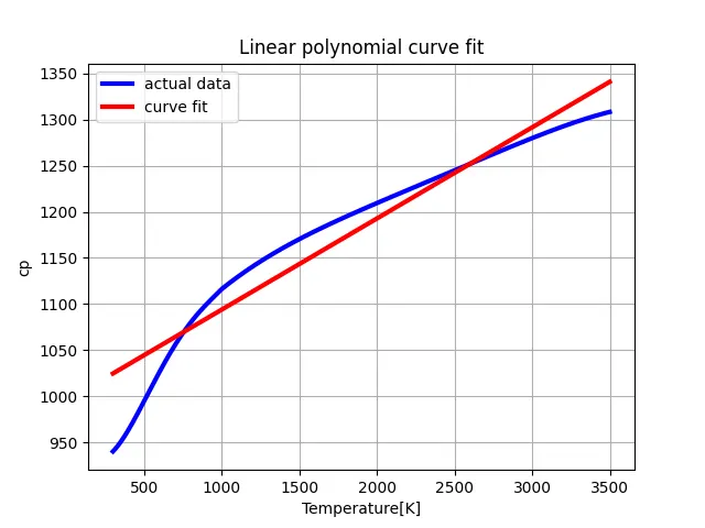
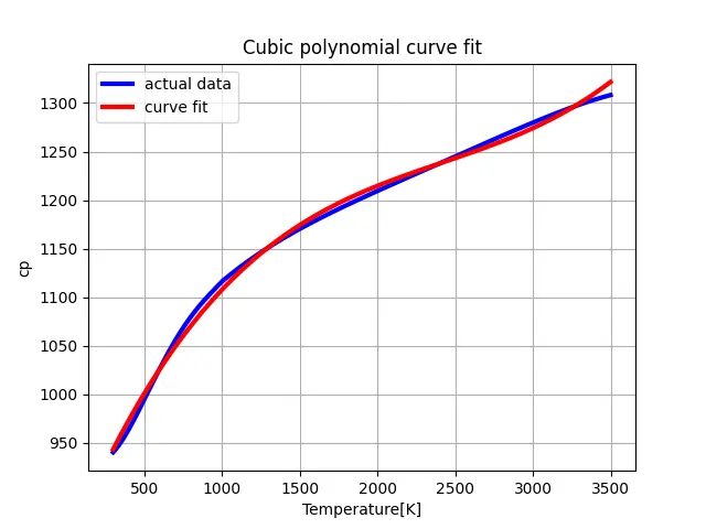
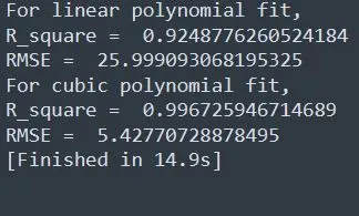
Here, from the above plottings, we say that the result obtained for the linear polynomial fit is R_square is 0.92 which we can say it as best fit and whereas the result obtained for the cubic polynomial fit is R_square is 0.99 which we can say it as a perfect fit. The RMSE value obtained is 5.42 which can be seen in the above result image.

5. What needs to be done in order to make the curve fit perfect?

Sol: In order to make the curve fit perfect we should increase the order of the polynomial then the rate of error will be less and the curve fit will be perfect. On increasing the order of the polynomial the value of R2will be close to 1 and it is assumed to the perfect fit.