Week 5 - Curve fitting

CURVE FITTING

Curve fitting is the process of constructing a curve that has the best fit to a series of data points. The curve fit can be used to find points anywhere along the curve hence can help one to predict future values.

Curve fitting involves interpolation and smoothing. Interpolation is where an exact fit to the data is required. Smoothing involves constructing a function that approximates fits the data.

CHOOSING THE BEST FIT

The best fit in a curve fit is the one that has the smallest deviation from the original data set. Hence it has the least error. In order to categorize the degree of the best fit, the following formulae are used.

• Sum of squares due to error:(ssr)

`ssr=sum_(i=1)^n=((f(x)-Mean)^2)`

Where f(x) is the predicted data

• Sum of squared errors:(sse)

`sse=sum_(i=1)^n Er(i)^2`

Where er is the error.

• R Square=r: it measures how successful the fit is in explaining the variation of the data.

`r=(ssr)/(sst)`

Where sst=sse+ssr

R square is a value between 0 and 1

Four programs are written for curve fitting using Python.

1. Linear curve fit
2. Cubic curve fit

Linear curve fit

Code

#Aurthor Arthur
#Linear Curve fitting using python

import math
import matplotlib.pyplot as plt
import numpy as np
from scipy.optimize import curve_fit

#Defining function 1 which is a polynomial of degree 1
#The function returns the equation of a straight line
def func_1(t,a,b):
    return a*t+b

#Definig function 2 which reads the text file data
def func_read():
    temp=[]
    cp=[]

    for line in open('data','r'):
        val=line.split(',')
        temp.append(float(val[0]))
        cp.append(float(val[1]))

    return[temp,cp]

#Storing the temp and cp as float arrays from the text files
temp,cp=func_read();


popt,pcov=curve_fit(func_1,temp,cp)
cp_1=func_1(np.array(temp),*popt)

#Finding mean of Cp data.

s=np.sum(cp)
l=np.size(cp)
m=s/l

# Calculating sum of squares

linearSse=0
linearSsr=0

for i in range(l):
    linearError=abs((np.sum((cp[i]-cp_1[i]))))
    linearSse=linearSse+pow(linearError,2)
    linearSsr=linearSsr+np.sum(pow((cp_1[i]-m),2))

linearSst=linearSse+linearSsr
print('linear_sst: ',linearSst)
linearR2=linearSsr/linearSst
print('Linear R2',linearR2)
linearRmse=pow((linearSse/l),0.5)
print('Linear_RMSE',linearRmse)


#Ploting the results
plt.figure(1)
plt.plot(temp,cp,'k--')
plt.plot(temp,cp_1,color='blue',linewidth=1)
plt.legend(['Actual data','Curve fit'])
plt.xlabel('Temprature(K)')
plt.ylabel('Cp')
plt.title('Linear Curve fitting')
plt.show()

Plot

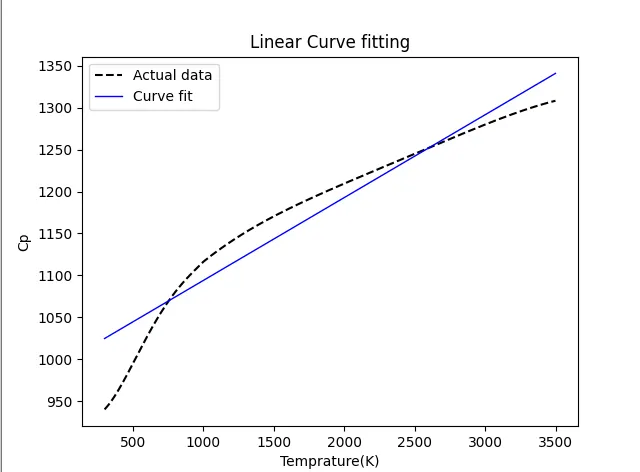
Linear curve fitting is when the data is fit to a straight line. The equation for a straight line is y=mx+c. Hence our aim is to calculate the values of x and y which will give us the best fit. From the graph, the line intersects the curve at two points.

From the code, the values of Sst, R square and Rmse are calculated and given below.

CUBE CURVE FITTING

#Aurthor Arthur
#Cube Curve fitting using python

import math
import matplotlib.pyplot as plt
import numpy as np
from scipy.optimize import curve_fit


#The function returns the equation of a plynomial of degree 3
def func_2(t,a,b,c,d):
    return a*pow(t,3)+b*pow(t,2)+c*t+d

#Definig function 2 which reads the text file data
def func_read():
    temp=[]
    cp=[]

    for line in open('data','r'):
        val=line.split(',')
        temp.append(float(val[0]))
        cp.append(float(val[1]))

    return[temp,cp]

#Storing the temp and cp as float arrays from the text files
temp,cp=func_read();

#Calculating the values cp2
popt,pconv=curve_fit(func_2,temp,cp)
cp_2=func_2(np.array(temp),*popt)

#Ploting the results
plt.figure(2)
plt.plot(temp,cp,'k--')
plt.plot(temp,cp_2,color='red',linewidth=1)
plt.legend(['Actual data','Curve fit'])
plt.xlabel('Temprature(K)')
plt.ylabel('Cp')
plt.title('Polynomial Curve fitting')
plt.show()

#Finding mean of Cp data.

s=np.sum(cp)
l=np.size(cp)
m=s/l

# Calculating sum of squares
#For cubic curve fit
cubicSse=0
cubicSsr=0

for j in range(l):
    cubicError=abs(np.sum((cp[j]-cp_2[j])))
    cubicSSe=cubicSse+pow(cubicError,2)
    cubicSsr=cubicSsr+np.sum(pow((cp_2[j]-m),2))


cubicSst=cubicSse+cubicSsr
print('Cubic SST: ',cubicSst)
cubicR2=cubicSsr/cubicSst
print('Cubic R2: ',cubicR2)
cubicRmse=pow((cubicSse/l),0.5)
print('cubic Rmse: ',cubicRmse)

Polynomial curve fitting is when a polynomial equation is used for fitting data. From the plot below the polynomial used was sufficient to fit the data.

PLOT

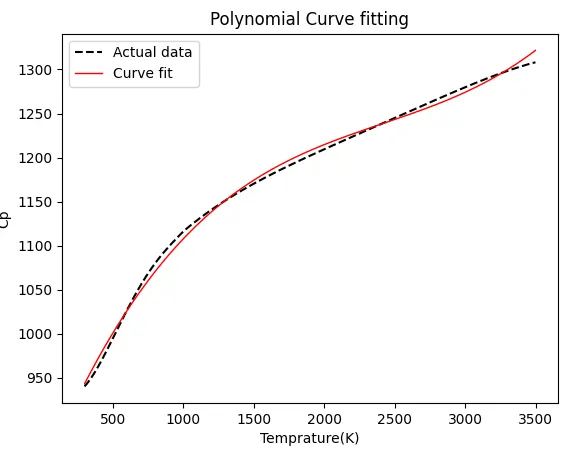
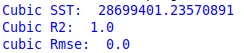
From the code, the values of Sst, R square and Rmse are calculated and given below.

Code explanation

1 . Important libraries are imported.

• matplot to allow plotting of figures
• math library for working with math functions such as cos, power.
• plotly library to enable working with graphs and tables.
• from scipy.optimize import curve_fit : Contains libraries for scientific and data analysis. For this case, we import curve fitting tools and libraries. Such as popt and pconv.

2.We create functions ie func_1 returns linear equation and func_2 returns the polynomial of degree 3.

3.Raw data is loaded and opened using func_read. Each line is read using a loop then the string is split and its data is stored in a temp and cp array.

4.From the function of reading the data we are able to get the temp and cp array.

5.For curve fitting popt and pcov are used as output for parameters obtained by curve fit. popt and pcov are tools from scipy library for curve fitting. The output is stored in cp_1 for the linear curve fit and cp_2 for polynomial curve fit.

6.Plots using original and the calculated data are created using matplot lib.

7. To calculate the fitness characteristics the equations of ssr , sst , sse and rmse are used as explained above.

Q AND A

1. What do popt and pcov mean?

Optimal values for the parameters so that the sum of the squared residuals off f(xdata, *popt) - y data is minimised.

'pcov' represents the square matrix that stores the estimated values of covariance of the coefficients above. The diagonal element of this square matrix also represents the variance of that coefficients.