Week 5 - Curve fitting

Python Program to Curve a given data set (Temperature and Cp)

Aim:

• Curve fit the given data set using the built-in curve fit function.
• Fit using linear and cubic polynomials
• Empirically find out the fit of the fitted with respect to the given data

Steps to code:

• Read the data and separate the temperature, Cp values into separate arrays using line split.
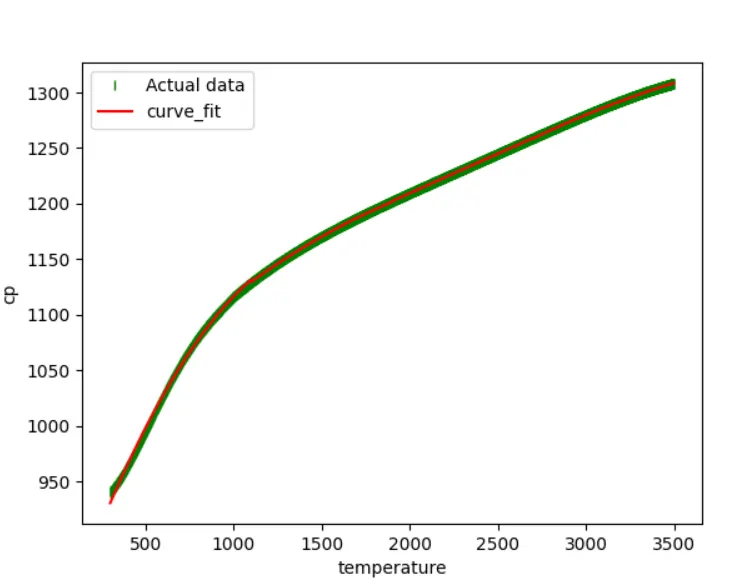
• To fit better, the data set is divided into 4 parts.
• Using the curve fit function, coefficients of the popt are found out.
• A for loop is used to iterate through the 4 data sets and using the coefficients, the function to fit data is called.
• Then all 4 sets are concatenated.
• To validate the goodness of the curve fit, the R square is method is used.

Note :

1. popt gives the coefficients of the function which fit the curve, pcov variable contains the covariance matrix, which indicates the uncertainties and correlations between parameters. This is most useful when the data has uncertainties.
2. np.array(temperature) store the temperatures data as NumPy array which is required as input for curve fit function

import numpy as np
import matplotlib.pyplot as plt
from scipy.optimize import curve_fit

from scipy import stats

def f(t,a,b,c):
	return a*pow(t,2) + b*t + c # fit the curve to represent this function



def read_file():
	temperature = []
	cp = []

	for line in open('data','r'): # opening the file and read
		values = line.split(',') # splitting the rows into based on commas
		temperature.append(float(values[0])) # save the temp and cp values in separate arrays
		cp.append(float(values[1]))

	return[temperature,cp]

temperature,cp = read_file() # calling the function

# np.savetxt("temp.csv", temperature, delimiter=",")

# np.savetxt("cp.csv", cp, delimiter=",")

four_way_split_temp = np.array_split(temperature,4) # splitting the array into 4 

four_way_split_cp = np.array_split(cp,4)

fit_cp = np.array([])

# print('temperature split',len(four_way_split_temp))

for i in range(len(four_way_split_temp)):


	popt, pcov = curve_fit(f,four_way_split_temp[i],four_way_split_cp[i]) # getting the coeffs

	print('coeff are :',popt)

	for coeff in popt:

		f_cp = f(np.array(four_way_split_temp[i]),*popt) # getting the fitted curve , passing the values of temp and coeff
		
		
	fit_cp = np.concatenate([fit_cp,f_cp]) # getting back the 4 way split into one array 

print("Data points are",len(fit_cp))



slope, intercept, r, p, std_err = stats.linregress(temperature, fit_cp) # in buillt function to the regression values

# empirical method to calculate the r square value
y_residue = cp - fit_cp

sse = sum(pow(y_residue,2))

ssr = sum(pow(fit_cp - np.mean(cp),2))

print('ssr',ssr)

print('sse',sse)

sst = ssr + sse

r_square = ssr/sst

print('empiral calculation of r_2 =' , r_square)
print("regression from using python lib ", r)

plt.plot(temperature,cp,'|',color= 'green',)
plt.plot(temperature,fit_cp,color= 'red')
plt.legend(['Actual data','curve_fit'])
plt.xlabel('temperature')
plt.ylabel('cp')
plt.show()


	

Linear and Cubic Fit Code:

import numpy as np
import matplotlib.pyplot as plt
from scipy.optimize import curve_fit
from scipy import stats

def read_file(): # reading the file and appending to separate arrays
	temperature = []
	cp = []

	for line in open('data','r'):
		values = line.split(',')
		temperature.append(float(values[0]))
		cp.append(float(values[1]))

	return[temperature,cp]

temperature,cp = read_file()

p_1 = np.polyfit(temperature,cp,1) # getting coeffs
p_3 = np.polyfit(temperature,cp,3)

fit_cp_1 = np.polyval(p_1,temperature) # getting the fitted curve valued for linear and cubic
fit_cp_3 = np.polyval(p_3,temperature)

y_residue_1 = cp - fit_cp_1
y_residue_3 = cp - fit_cp_3

sse_1 = sum(pow(y_residue_1,2))
sse_3 = sum(pow(y_residue_3,3))

ssr_1 = sum(pow(fit_cp_1 - np.mean(cp),2))
ssr_3 = sum(pow(fit_cp_3 - np.mean(cp),2))

sst_1 = ssr_1 + sse_1
sst_3 = ssr_3 + sse_3

r_square_1 = ssr_1/sst_1
r_square_3 = ssr_3/sst_3

print('linear fit empiral calculation of r_2 =' , r_square_1)
print('cubic fit empiral calculation of r_2 =' , r_square_3)


plt.plot(temperature,cp,color= 'blue',)
plt.plot(temperature,fit_cp_1,color= 'red')
plt.title("Linear Fit") 

message = str(r_square_1)

plt.legend(['Actual data','curve_fit_linear','message'])
plt.xlabel('temperature')
plt.ylabel('cp')
plt.show()

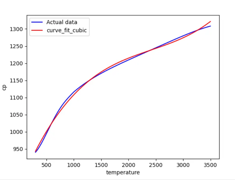
plt.plot(temperature,cp,color= 'blue',)
plt.plot(temperature,fit_cp_3,color= 'red')
plt.legend(['Actual data','curve_fit_cubic'])
plt.xlabel('temperature')
plt.ylabel('cp')
plt.show()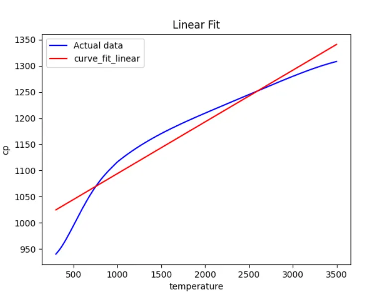

Results:

The Regression values obtained from the linear and cubic fits are:

The cubic fits gave a better fit than linear fit.

The empirically calculated regression value obtained from the first program is 0.999, the curve fit function was manually given into the curve fit function.

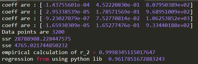
In order to make the fit more correct, the data set can be divided into smaller sets to get hold of the complexities in the curve and then concatenated, also polynomials with more degrees can be used to get better fit.