Week 5 - Curve fitting
#Objective: Write a program in python which gives best curve fit function for given data set.
#Introduction:
Curve fitting:
Curve fitting is the process of specifying the model that provides the best fit to the specific curves in your dataset. Curved relationships between variables are not as straightforward to fit and interpret as linear relationships.
For linear relationships, as you increase the independent variable by one unit, the mean of the dependent variable always changes by a specific amount. This relationship holds true regardless of where you are in the observation space.
Unfortunately, the real world isn’t always nice and neat like this. Sometimes your data have curved relationships between variables. In a curved relationship, the change in the dependent variable associated with a one unit shift in the independent variable varies based on the location in the observation space. In other words, the effet of the independent variable is not a constant value.
-----------------------------------------------*************************----------------------------------
1. What does popt and pcov mean?
Ans.popt-The return value contains the best-fit values of the parameters.
pcov-The return value pcov contains the covariance (error) matrix for the fit parameters. From them we can determine the standard deviations of the parameters.
---------------------------------------------*************************-----------------------------------
2. What does np.array(temperature) do?(shown in video)
Ans.From the pic shown below:

Function'fun' is called giving 'temperature' ,which is a list of temperature values extracted from data file provided.
and that function'fun' return value (a*pow(t,2)+b*t+c).
This pow() inbuilt function do not accept list as input,therefore it is giving error.
For eliminating this error,we have to convert 'temperature' list into numpy array by using 'np.array(temperature)'
------------------------------------------------*********************-------------------------------------
3. What does the *popt mean in program.
Ans. As we know from the program,popt contains best fit values of parameters(like a,b,c etc given in program).We passed *popt as a value to the function 'fun' while calling it.
--------------------------------------------*************************------------------------------------
4.Write code to fit a linear and cubic polynomial for the Cp data. Explain if your results are good or bad.
Ans.Program include R square calculation for Linear and Cubic function.
"""
Curve fit challenge linear and cubic curve fit program

"""
import numpy as np
import matplotlib.pyplot as plt
from scipy.optimize import curve_fit


#Curve ft function for linear polynomial
def func(t,a,b,):
	return a*t+b


#Curve ft function for linear polynomial
def func1(t,a,b,c,d):
	return a*pow(t,3)+b*pow(t,2)+c*t+d


#Reading thermodynamic data file
def read_file():
	temperature=[]
	cp=[]
	for line in open('data','r'):
		values=line.split(',')
		temperature.append(float(values[0]))
		cp.append(float(values[1]))

	return (temperature,cp)


#Main program
temperature,cp=read_file()

popt,pcov =curve_fit(func,temperature,cp)
fit_cp=func(np.array(temperature),*popt)						#temperature array and constants passed through popt

popt1,pcov1 =curve_fit(func1,temperature,cp)
fit_cp1=func1(np.array(temperature),*popt1)						#temperature array and constants passed through popt1

plt.figure(1)
plt.plot(temperature,cp,color='blue',linewidth=3,label='Actual curve')
plt.plot(temperature,fit_cp,color='red',linewidth=3,label='Linear curve fit func')
plt.xlabel('Temperature(kelvin)')
plt.ylabel('Specific heat(Cp)(in J/(kg-K)')
plt.title('Plot between Temperature and specific heat')
plt.legend(loc='lower right')

plt.figure(2)
plt.plot(temperature,cp,color='blue',linewidth=3,label='Actual curve')
plt.plot(temperature,fit_cp1,color='green',linewidth=3,label='Cubic curve fit func')
plt.xlabel('Temperature(kelvin)')
plt.ylabel('Specific heat(Cp)(in J/(kg-K)')
plt.title('Plot between Temperature and specific heat')
plt.legend(loc='lower right')


"""
R^2 value calculation for linear function
"""

#Arithmetic Mean of cp values given in data file
Mean_cp_value=sum(cp)/len(cp)

# Calculation of Ssr(Sum of square of regression) for linear curve fit function
ssr_linear=0

for j in range(len(cp)):
	cp_diff_linear=pow((fit_cp[j]-Mean_cp_value),2)
	ssr_linear=ssr_linear+cp_diff_linear

# Calculation of Sse(Sum of square due to error) for linear curve fit function
sse_linear=0

for k in range(len(cp)):
	cp_diff_act_curvefit=pow((cp[k]-fit_cp[k]),2)
	sse_linear=sse_linear+cp_diff_act_curvefit

#Defining Sst
sst_linear=ssr_linear+sse_linear

#Calculating R^2
R_square_linear=ssr_linear/sst_linear
print('R square value for linear curve fit : {0}'.format(R_square_linear))


"""
R^2 value calculation for cubic function
"""

# Calculation of Ssr(Sum of square of regression) for cubic curve fit function
ssr_cubic=0

for j in range(len(cp)):
	cp_diff_cubic=pow((fit_cp1[j]-Mean_cp_value),2)
	ssr_cubic=ssr_cubic+cp_diff_cubic

# Calculation of Sse(Sum of square due to error) for cubic curve fit function
sse_cubic=0

for k in range(len(cp)):
	cp_diff_act_curvefit_cubic=pow((cp[k]-fit_cp1[k]),2)
	sse_cubic=sse_cubic+cp_diff_act_curvefit_cubic

#Defining Sst
sst_cubic=ssr_cubic+sse_cubic

#Calculating R^2
R_square_cubic=ssr_cubic/sst_cubic
print('R square value for cubic curve fit : {0}'.format(R_square_cubic))

plt.show()
#Plots:
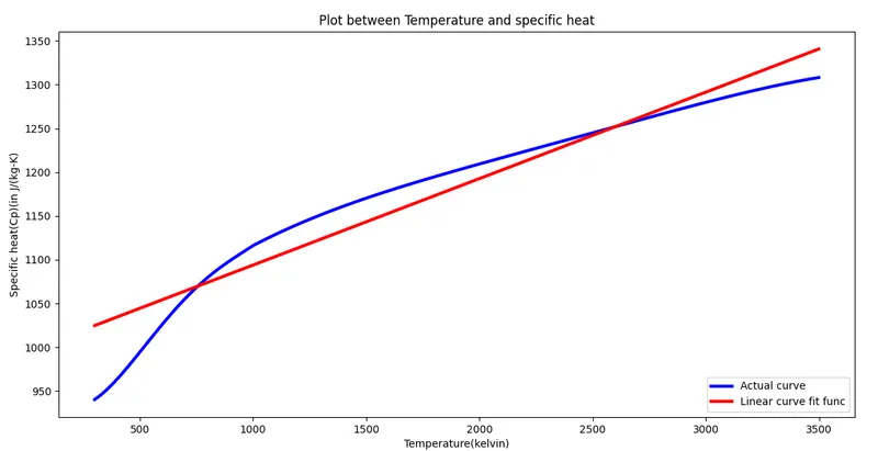
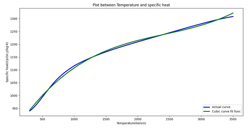
From both the above plots ,it can be noticed that linear curve fit function only match or fit at only two points.And cubic curve fit function comes out to fit in a better way.
But as the order of polynomial increases,the value of dependent variable changes rapidly even for little change in independent variable value.Therefore error associated would also increase.
So it should be tried to match curve fit function of lower order.
--------------------------------------------------***************---------------------------------------------
5. What needs to be done in order to make the curve fit perfect.
Ans.As we saw even in cubic curve fit function,actual fit values were still not matching completely because whole data is chosen in only one region.
So in 2 ways we can make curve fit perfect:
a.)Splitting the data values into several regions:So the range of each data region would be small,which would fit better than selecting one region for whole data values.
b.)Keeping the order of curve fit function as lower as possible:As the order of polynomial increases,error associated with the curve fit function also increases.
#Program implementing above 2 correction steps is given below:Include R square calculation for region 1.
"""
Curve fit challenge quadratic curve fit program

"""

import numpy as np
import matplotlib.pyplot as plt
from scipy.optimize import curve_fit

#Curve ft function
def func(t,a,b,c):
	return a*pow(t,2)+b*t+c


#Reading thermodynamic data file
def read_file():
	temperature=[]
	cp=[]
	for line in open('data','r'):
		values=line.split(',')
		temperature.append(float(values[0]))
		cp.append(float(values[1]))

	return (temperature,cp)

#Main program
temperature,cp=read_file()

#Temperature array defined
temp_array=np.array(temperature)

#C_p array defined
cp_array=np.array(cp)

#Temperature and cp array defined for different temperature regions.
temp_array1=temp_array[temp_array<=500]
cp_temp_array1=cp[0:len(temp_array1)]

temp_array2=temp_array[(temp_array> 500) & (temp_array <= 1000)]
cp_temp_array2=cp_array[(np.where((temp_array> 500) & (temp_array <= 1000)))]

temp_array3=temp_array[(temp_array> 1000) & (temp_array <= 1500)]
cp_temp_array3=cp_array[(np.where((temp_array> 1000) & (temp_array <= 1500)))]

temp_array4=temp_array[(temp_array> 1500) & (temp_array <= 2000)]
cp_temp_array4=cp_array[(np.where((temp_array> 1500) & (temp_array <= 2000)))]

temp_array5=temp_array[(temp_array> 2000) & (temp_array <= 2500)]
cp_temp_array5=cp_array[(np.where((temp_array> 2000) & (temp_array <= 2500)))]

temp_array6=temp_array[(temp_array> 2500) & (temp_array <= 3000)]
cp_temp_array6=cp_array[(np.where((temp_array> 2500) & (temp_array <= 3000)))]

temp_array7=temp_array[(temp_array> 3000)]
cp_temp_array7=cp_array[(np.where(temp_array> 3000))]


popt1,pcov1 =curve_fit(func,temp_array1,cp_temp_array1)
fit_cp1=func(temp_array1,*popt1)


popt2,pcov2 =curve_fit(func,temp_array2,cp_temp_array2)
fit_cp2=func(temp_array2,*popt2)


popt3,pcov3 =curve_fit(func,temp_array3,cp_temp_array3)
fit_cp3=func(temp_array3,*popt3)

popt4,pcov4 =curve_fit(func,temp_array4,cp_temp_array4)
fit_cp4=func(temp_array4,*popt4)

popt5,pcov5 =curve_fit(func,temp_array5,cp_temp_array5)
fit_cp5=func(temp_array5,*popt5)

popt6,pcov6 =curve_fit(func,temp_array6,cp_temp_array6)
fit_cp6=func(temp_array6,*popt6)

popt7,pcov7 =curve_fit(func,temp_array7,cp_temp_array7)
fit_cp7=func(temp_array7,*popt7)


plt.plot(temperature,cp,color='blue',linewidth=3,label='Actual curve')
plt.plot(temp_array1,fit_cp1,color='red',linewidth=3,label='Region-1-Quad. curve fit func')
plt.plot(temp_array2,fit_cp2,color='green',linewidth=3,label='Region-2-Quad. curve fit func')
plt.plot(temp_array3,fit_cp3,color='yellow',linewidth=3,label='Region-3-Quad. curve fit func')
plt.plot(temp_array4,fit_cp4,color='black',linewidth=3,label='Region-4-Quad. curve fit func')
plt.plot(temp_array5,fit_cp5,color='pink',linewidth=3,label='Region-5-Quad. curve fit func')
plt.plot(temp_array6,fit_cp6,color='brown',linewidth=3,label='Region-6-Quad. curve fit func')
plt.plot(temp_array7,fit_cp7,color='green',linewidth=3,label='Region-7-Quad. curve fit func')

plt.xlabel('Temperature(kelvin)')
plt.ylabel('Specific heat(Cp)(in J/(kg-K)')
plt.title('Plot between Temperature and specific heat')
plt.legend(loc='lower right')


"""
R^2 value calculation for quadratic function region1 Temperature below 500
"""

#Arithmetic Mean of cp values given in data file
Mean_cp_value1=sum(cp_temp_array1)/len(cp_temp_array1)

# Calculation of Ssr(Sum of square of regression) for quadratic curve fit function
ssr_quad1=0

for j in range(len(cp_temp_array1)):
	cp_diff_quad1=pow((fit_cp1[j]-Mean_cp_value1),2)
	ssr_quad1=ssr_quad1+cp_diff_quad1

# Calculation of Sse(Sum of square due to error) for quadratic curve fit function
sse_quad1=0

for k in range(len(cp_temp_array1)):
	cp_diff_act_curvefit_quad1=pow((cp_temp_array1[k]-fit_cp1[k]),2)
	sse_quad1=sse_quad1+cp_diff_act_curvefit_quad1

#Defining Sst
sst_quad1=ssr_quad1+sse_quad1

#Calculating R^2
R_square_quad1=ssr_quad1/sst_quad1
print('R square value for quad curve fit region 1 : {0}'.format(R_square_quad1))

plt.show()
#Plot obtained from above program:
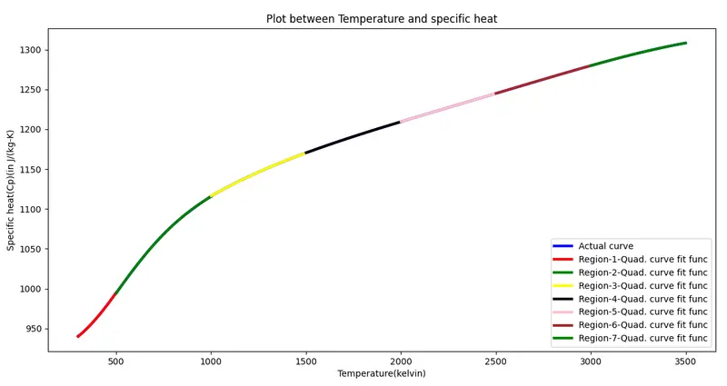
From the plot ,it can be concluded that curve fit is perfect.
--------------------------------------------*************************-------------------------------------
6. Show empirically as to how well your curve has been fit.
Ans.To empirically show,curve fit is perfect or how good it has been fit,we need to calculate R square value for curve fit function.
R square:
R-square is a statistical measure of how close the data are to the fitted regression line. It is also known as the coefficient of determination, or the coefficient of multiple determination for multiple regression.
Like we calculated R square value for all Linear,Quadratic (region1),Cubic.
So for Linear ,R square came out be least,then for cubic curve fit function choosing whole data at once.
But after splitting and using quadratic function,R square came out to be more than cubic curve fit function.
##R square calculation has been included in the program##
---------------------------------------------********************-------------------------------------------