CURVE FITTING WITH ORIGINAL DATA BY USING POLYNOMIALS IN PYTHON

AIM

To create the predicted curve for fiitting with original data curve in perfectly eachother by using polynomial equations, is to do in PYTHON.

INTRODUCTION

Curve fitting is the process of constructing a curve, or mathematical function, that has the best fit to a series of data points, possibly subject to constraints. Curves such as parabola and hyperbola are used in architecture to design arches in buildings. The purpose of curve fitting is to specify an appropriate function and adjust its parameters in a way that it matches, as close as possible, an experimental or historical data set. Fitting functions can be derived by applying regression techniques, interpolation, and spline curves.

Curve fiitting is help to predicting future values at specific point. For example, predicting the population growth at next year, predicting share markets scenario and so on.

Robust curve fitting

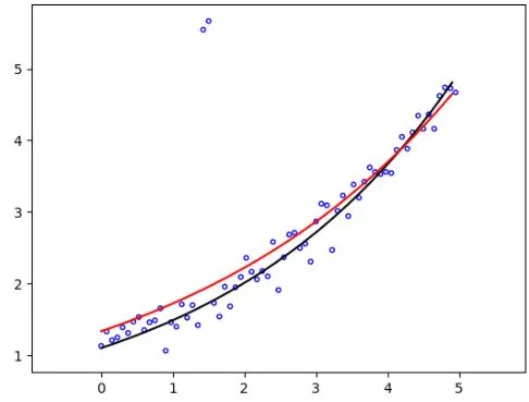
This figure represents the curve fitting the black color curve is raw data curve, the red color curve is predicted curve by using polynomial curve. To increase the degree of polynomial, the red colour curve will exactly fit into the black colour curve. This is called curve fitting.

OBJECTIVES

1) To create a python code for finding the perfect curve fit by using linear and cubic polynomials.

2) Check it goodness of fit criteria for individual polynomial equation.

3) Plot results should be comparing to both predicted and original curve.

WHAT IS POLYNOMIALS

A ploynomial is an expression of more than one algebraic terms, especially of several terms that contains different powers of the same variables.

Types of polynomials equation

Linear equation

`Y = a(T)+b`

It plotted on a graph, it's actually in exactly straight line. Typically, it is directly proportional to indenpendent variables.

Quadratic equation

`Y = a(T)^2 + b(T) + c`

It plotted on a graph, it's looks parabolic curve.

Cubic equation

`Y = a(T)^3 +b(T)^2 + c(T) + d`

It plotted on a graph, it's looks cubic curve.

n th order equation

`Y = P1(T)^(n) + P2(T)^(n-1) + ......+Pn-1(T)+Pn`

It plotted on a graph, it's looks nonlinear curve.

QUALITIES FOR FINDING THE GOODNESS OF FIT CRITERIA

1) Sum of squares due to error (SSE)

2) R - square

3) Adjustive R - square

4) Root mean squared error (RMSE)

Sum of squared error

SSE is the sum of squared deviations of actual value from the predicted values. The SSE value is 0, the predicted curve fit is exactly fitted overlapped the original raw data curve. The SSE value is too high, that means the predicted value does not correct fit. So, we increase the ploynomial when the curve is fitted over the raw data curve.

Formula to finding the sum of squared error.

`SSE = sum_(i=1)^n (Y(i) - f(x(i)))^2`

Sum of squared regression

SSR is the sum of squared of predicted values from the mean value. The SSR value are 0 or high, same previous scenario is held on in sum of squared regression.

Formula to finding the sum of squared regression.

`SSR = sum_(i=1)^n (f(x(i))-Mean)^2`

Total sum of square

The total sum of squares is the addition of sum of sqaured error and sum of squared regression.

`SST = SSE +SSR`

R - Square

R - square value is a sum of squared regression upon total sum of square

`R ^2 = (SSR)/(SST)`

The value of R square is 0, it is very bad fit. The value of R square is 1, it is very good fit.

Acceptable R square values

0.3 < r < 0.5 this value is generally considered a weak or low effect size.

0.5 < r< 0.7 this value is generally considered a moderate effect size.

r > 0.7 this value is generally considered a strong effect size and it is recommended for best R square values.

Adjusted R - square

The adjusted R-squared is a modified version of R-squared that has been adjusted for the number of predictors in the model. The adjusted R-squared increases only if the new term improves the model more than would be expected by chance.

It depends on independent variables, it is negligible infinitesimal variation from R square.

`1 - [((1-R^2)(n-1))/(k-1)]`

Where,

n = Number of data points

k = Number of independent variables

Root mean square error

Root mean square error (RMSE) is the standard deviation of the residuals (predicted errors). Residuals are a measure of how far from the regression line data points are; RMSE is a measure of how spread out these residuals are. In other words, it tells you how concentrated the data is around the line of best fit.

`sqrt(((sum_(i=1)^2)(Y(i) - f(x(i)))^2)/n)`

`sqrt((SSE)/n)`

QUESTIONS AND ANSWERS

What does popt and pcov mean ?

1) Popt is basically to finding optimal coefficient values for which desired equations such as linear, quadratic, cubic and N number of polynomial. This coefficient values are calculating from curve_fit function with desired equation function, Specific heat of given gas and temperature. So that sum of squared residuals or error will be minimized.

Popt for linear equation have 2 constant coefficients such as a & b. Popt for cubic equation have 4 constant coefficients such as a,b,c & d.

2) Pcov is basically covariance of popt. A values are stored in the form of 2d array(that means matrix format), a diagonals provide of the coefficient estimate.

Pcov for linear equation have 4 constant co-coefficients. Pcov for cubic eqaution have 16 constant Co-coefficients.

What does np.array(temperature) do ?

A Numpy module is usually handling the array or list, in order extract the one by one temperature value from temperature array to passing into respective equation like linear or cubic through which corresponding function

What does the in *popt mean?

A asterisk(*) symbol is helps us to refers the coefficients value for which respective equations.

What needs to be done in order to make the curve fit perfect?

Increase the order of polynomial to when the predicted curve will perfectly match to actual curve or else split the orginal data points at different ranges, write a python code in proper manner to get achieve the curve fit without increasing the polynomial of equation.

Show empirically as to how well your curve has been fit ?

By observation, a cubic predicted curve has been almost fit into original data curve with some tolerance compared to linear predicted curve. If curve fit overlapped to original data with comes under the defined some tolerances, it is called best fit.

The perfect fit is always a best fit, but the best fit is not a perfect fit.

PYTHON CODE :

import numpy as np 
import matplotlib.pyplot as plt 
from scipy.optimize import curve_fit
from statistics import mean

# Linear fit function
def linear(t,a,b):
	return a*t + b

# Cubic fit function
def Cubic(t,a,b,c,d):
	return a*pow(t,3) + b*pow(t,2) +c*t + d

#Reading thermodynamic data file

def read_file():
	temperature = []
	Cp = []
	
	for line in open('data','r'):
		values = line.split(',')
		temperature.append(float(values[0]))
		Cp.append(float(values[1]))
	return[temperature,Cp]


# Main program
temperature,Cp = read_file()
popt1,pcov1 = curve_fit(linear,temperature,Cp)
popt2,pcov2 = curve_fit(Cubic,temperature,Cp)
fit_cp1 = linear(np.array(temperature),*popt1)
fit_cp2 = Cubic(np.array(temperature),*popt2)


plt.figure()
plt.plot(temperature,Cp,color = "blue", linewidth = 3)
plt.plot(temperature,fit_cp1,color = "red", linewidth = 3)
plt.legend(['Actual data','Linear fit'])
plt.xlabel('Temperature in Kelvin')
plt.ylabel('Specific Heat in Kj/kg K')
plt.title('Actual curve with linear curve')
plt.savefig('Actual curve with linear curve')
plt.show()

plt.figure()
plt.plot(temperature,Cp,color = "blue", linewidth = 3)
plt.plot(temperature,fit_cp2,color = "red", linewidth = 3)
plt.legend(['Actual data','Cubic fit'])
plt.xlabel('Temperature in Kelvin')
plt.ylabel('Specific Heat in Kj/kg K')
plt.title('Actual curve with Cubic curve')
plt.savefig('Actual curve with Cubic curve')
plt.show()

plt.figure()
plt.plot(temperature,Cp,color = "blue", linewidth = 3)
plt.plot(temperature,fit_cp1,color = "red", linewidth = 3)
plt.plot(temperature,fit_cp2,color = "green", linewidth = 3)
plt.legend(['Actual data','Linear fit','Cubic feet'])
plt.xlabel('Temperature in Kelvin')
plt.ylabel('Specific Heat in Kj/kg K')
plt.title('Actual curve with both linear & Cubic curve')
plt.savefig('Actual curve with both linear & Cubic curve')
plt.show()

# Storing the SSE and SSR for both linear and cubic
SSE_1 = []
SSE_2 = []
SSR_1 = []
SSR_2 = []

for i in range(0,len(Cp)):

	ct = 0
	Avg = mean(Cp)	
	
	a = Cp[i] - fit_cp1[i]
	b = Cp[i] - fit_cp2[i]
	c = fit_cp1[i] - Avg
	d = fit_cp2[i] - Avg


	SSE_1.append(pow(a,2))
	SSE_2.append(pow(b,2))
	SSR_1.append(pow(c,2))
	SSR_2.append(pow(d,2))
	
	ct = ct + 1

# Finding goodness of fit criteria
SSE_linear = sum(SSE_1)
SSE_cubic = sum(SSE_2)
SSR_linear = sum(SSR_1)
SSR_cubic = sum(SSR_2)


SST_linear = SSE_linear + SSR_linear
SST_cubic = SSE_cubic + SSR_cubic

R_square_linear = (SSR_linear)/(SST_linear)
R_square_cubic = (SSR_cubic)/(SST_cubic)


n = 3200
k = 3200

R_Square_Adjustable_Linear = 1 - (((1-R_square_linear)*(n-1))/(k - 1))
R_Square_Adjustable_Cubic = 1 - (((1-R_square_cubic)*(n-1))/(k - 1))

RSME_Linear = pow(((SSE_linear)/n),0.5)
RSME_Cubic = pow(((SSE_cubic)/n),0.5)

# Printing goodness of fit criteria values
print('Sum of sqaure due to error for linear =',SSE_linear)
print('Sum of sqaure due to error for Cubic =',SSE_cubic)
print('Sum of square of regression for linear =',SSR_linear)
print('Sum of square of regression for Cubic =',SSR_cubic)
print('Total sum of square for linear =',SST_linear)
print('Total sum of square for linear =',SST_cubic)
print('R Square for linear =',R_square_linear)
print('R Square for Cubic =',R_square_cubic)
print('Adjustable R sqaure for linear =',R_Square_Adjustable_Linear)
print('Adjustable R sqaure for Cubic =',R_Square_Adjustable_Cubic)
print('Root Mean Square Error for linear =',RSME_Linear)
print('Root Mean Square Error for Cubic =',RSME_Cubic)

EXPLANATION :

1) Importing the neccessary modules such as numpy, matplotlib, curve fit from scipy optimize and mean from statistics.

2) Matplotlib modules is help us to plotting, numpy module is help to operting the arrays, mean module is help us to average the list and curve fit module is help us to finding the polynomial coefficients and finding the covariance of that polynomial.

3) Defining the functions for both linear equation and cubic equation and also create a function to extracting the temperature & Specific heat value from data file.

4) By using curve fit function to calculate the coefficients of polynomial & Covariance respective to type of polynomial euation. If we want to calculate those of the thing by using temperature, specific heat and respective function either linear or cubic.

5) After that, we calculated the predicted specific heat values in each and every temperatures for both linear and cubic equation.

6) We want to check the fit by uisng some goodness fit criteria like SSE, R Square, Rsquare Adjustable and RSME for both linear and cubic fit.

7) Print it down the order of goodness of fit criteria values and make a plot in separately.

RESULTS AND DISCUSSION :

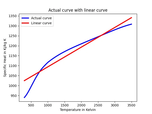
Actual Curve with linear curve :

To plotting the both actual data curve and linear curve on a single image. It clearly shown, a linear fit should not match with each other.

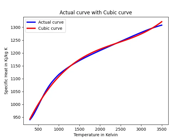
Actual data curve with cubic curve :

To plotting the both actual curve and cubic curve on a single image. It clearly shown, a cubic curve and original curve is almost match with eachother compared to linear predicted curve.

Superimposing the actual data curve and predicted curve for both linear & Cubic on a single plot.

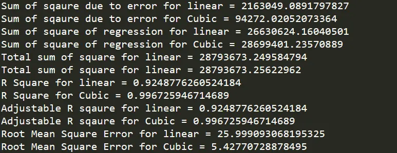
Goodness of fit criteria values are sort out the below snap. We concerned any one of the goodness fit, now take the R Square method to find out predicted curve either good or bad (1 is good and 0 is bad), a cubic R Square value is close to 1 compare to linear predicted curve. So that, A cubic curve fit is best fit from one of the goodness of fit criteria.

CONCLUSION :

A predicted cubic curve is almost overlapped with original data curve compared to linear predicted curve. So, Cubic curve is best curve fit.