Week 5 - Curve fitting
Curve Fitting Using Python
Aim:
* To perform a curve fitting for a given dataset of Temperature and Specific Heat capacity and to find the best and perfect fit for that particular dataset using python.
* To plot Linear and Cubic Fit curves from the given dataset and to find the perfect fit curve that exactly matches the Actual data.
Procedure:
* A curve fit is a mathematical function which has a relationship with a particular set of data points.
* It is used to describe how the data changes mathamatically. Fitted curves can be used as an aid for data visualization,and to summarize the relationships among two or more variables.
* There is a indipendent variable and a dependent variable in the dataset and when put in the curve fit mathematical expression we can get some rough results ,that is the values close to the exact result and based on the accuracy of the fit we can predict the results correctly.
* Here we are doing a program in python to find the best fit that can be used to predict the exact results for the dataset of Temperature 't' (K) and specific heat 'cp' (KJ/Kmol-K).
* The independent variable here is Temperature and dependent variable is specific heat.
* Now for performing a curve fit we need to use this dataset into an mathematical expression of any polynomial degrees (say) linear, quadratic, cubic or of (n)th order to figure out the coefficients and so it closely represents the original dataset.
* The Idea of curve fitting is basically fitting the Given dataset (Temperature & Cp) to the required Function (Linear & Cubic)
Linear = a*t + b
Cubic = a*t^3 + b*t^2 + c*t + d
* Then we can plot the values and see which polynomial closely represents the original dataset.
Parameters used to measure the fitness characteristics for both the curves:
* To find the fitness of the curve we are using 'Rsquare' method which can be used to predict the acuracy of the curve fit.
* To find the fitness of the determined curve fit we are using this method where, R-squared is a statistical measure of how close the data are to the fitted regression line.
* It is also known as the coefficient of determination or the coefficient of multiple determination for multiple regression.
R-squared = Explained variation / Total variation
Determining R^2:
If y = f(x) is the curve fitness then from the above diagram we can say,
R^2 = SSR/SST where,
SSR - Sum of squares of regression is a measure of the discrepancy between the data and an predicted data.
SSE - Sum of the squarred estimates of error
SST - Sum of the squared differences between the observations and their overall mean.
SST = SSR + SSE
* The value R2 quantifies goodness of fit. It is a fraction between 0.0 and 1.0, and has no units. Higher values indicate that the model fits the data better.
* When R2=1.0, all points lie exactly on the curve with no scatter that means , If you know X data points we can calculate the Y data point exactly, So the Curve variation can be calculated exactly for the future data points too.
* We can predict the further variation in the dependent variable Cp for the change in independent variable Temperature.
Python Coding :
# Importing required libraries for performing curve fit
import math
import numpy as np
import matplotlib.pyplot as plt
from scipy.optimize import curve_fit

# Defining the Linear and Cubic Functions
def linear_function(t,a,b):
	return a*t + b

def cubic_function(t,a,b,c,d):
	return a*pow(t,3) + b*pow(t,2) + c*t + d

# Defining Higher order polynomial functions of 5th and 8th degree for getting perfect fit

def quintic_function(t,a,b,c,d,e,f):
	return a*pow(t,5) + b*pow(t,4) + c*pow(t,3) + d*pow(t,2) + e*t + f

def octic_function(t,a,b,c,d,e,f,g,h,i):
	return a*pow(t,8) + b*pow(t,7) + c*pow(t,6) + d*pow(t,5) + e*pow(t,4) + f*pow(t,3) + g*pow(t,2) + h*t + i

# Reading the Given Temperature vs Specific heat Dataset from the file 'data'
def read_file():
	temperature = []
	cp = []
	for line in open('data','r'):
		value = line.split(',')
		temperature.append(float(value[0]))
		cp.append(float(value[1]))
	return [temperature,cp]

# Curve fitting the dataset to the function
temperature,cp = read_file()

# Linear Curve fitting
popt,pcov = curve_fit(linear_function,temperature,cp)
fit_cp_linear = linear_function(np.array(temperature), *popt)
plt.figure(1)
plt.plot(temperature,cp,'b--',linewidth = 2)
plt.plot(temperature,fit_cp_linear,'r',linewidth = 2)
plt.legend(['Actual Dataset','Predicted Dataset'])
plt.xlabel('Temperature (K)')
plt.ylabel('Specific Heat-cp (J/KgK)')
plt.title('Linear Curve Fit')
plt.show()

# Cubic Curve fitting
popt,pcov = curve_fit(cubic_function,temperature,cp)
fit_cp_cubic = cubic_function(np.array(temperature), *popt)
plt.figure(2)
plt.plot(temperature,cp,'b--',linewidth = 2)
plt.plot(temperature,fit_cp_cubic,'r',linewidth = 2)
plt.legend(['Actual Dataset','Predicted Dataset'])
plt.xlabel('Temperature (K)')
plt.ylabel('Specific Heat-cp (J/KgK)')
plt.title('Cubic Curve Fit')
plt.show()

# Measuring the fitness of the curve
'''
SSE (Sum of squares due to errors)
SSR (Sum of squares of Regression)
SST = SSE + SSR
R^2 = SSR / SST

Mean of CP Data
Mean = sum of all elements / Total number of elements

'''
Sum = np.sum(cp)
Length = np.size(cp)
Mean = Sum / Length
print('Mean of cp=',Mean)


linear_SSE = 0
linear_SSR = 0
for i in range(Length):
	linear_error = abs((np.sum((cp[i] - fit_cp_linear[i]))))
	linear_SSE = linear_SSE + pow(linear_error,2)
	linear_SSR = linear_SSR + np.sum(pow((fit_cp_linear[i] - Mean),2))

linear_SST = linear_SSE +linear_SSR
print('Linear SST =',linear_SST)
linear_R2 = linear_SSR / linear_SST
print('Linear R square =',linear_R2)

Cubic_SSE = 0
Cubic_SSR = 0
for i in range(Length):
	Cubic_error = abs((np.sum((cp[i] - fit_cp_cubic[i]))))
	Cubic_SSE = Cubic_SSE + pow(Cubic_error,2)
	Cubic_SSR = Cubic_SSR + np.sum(pow((fit_cp_cubic[i] - Mean),2))

Cubic_SST = Cubic_SSE +Cubic_SSR
print('Cubic SST =',Cubic_SST)
Cubic_R2 = Cubic_SSR / Cubic_SST
print('Cubic R square =',Cubic_R2)

# For finding perfect fit we use higher polynomial of degree '5' & '8'

# quintic Curve fitting
popt,pcov = curve_fit(quintic_function,temperature,cp)
fit_cp_quintic = quintic_function(np.array(temperature), *popt)
plt.figure(3)
plt.plot(temperature,cp,'b--',linewidth = 3)
plt.plot(temperature,fit_cp_quintic,'r',linewidth = 2)
plt.legend(['Actual Dataset','Predicted Dataset'])
plt.xlabel('Temperature (K)')
plt.ylabel('Specific Heat-cp (J/KgK)')
plt.title('Quintic Curve Fit')
plt.show()

# Octic Curve fitting
popt,pcov = curve_fit(octic_function,temperature,cp)
fit_cp_octic = octic_function(np.array(temperature), *popt)
plt.figure(4)
plt.plot(temperature,cp,'b--',linewidth = 3)
plt.plot(temperature,fit_cp_octic,'r',linewidth = 2)
plt.legend(['Actual Dataset','Predicted Dataset'])
plt.xlabel('Temperature (K)')
plt.ylabel('Specific Heat-cp (J/KgK)')
plt.title('Octic Curve Fit')
plt.show()
* First all the required libraries like math, numpy, scipy, to perform curve fitting is imported into the program.
* Then the Function in which we need the dataset is defined. In this case Linear and Cubic Functions are defined.
* Then we are defining a function for Reading the Given Temperature vs Specific heat capacity Dataset from the file 'data'. Then the string values extracted are converted to float variables are are stored in individual arrays namely, Temperature and Cp.
* Then we are performing the curve fitting by calling the dataset read and the Function defined into the 'Curve_fit' command.
* In this line of code, " popt,pcov = curve_fit(linear_function,temperature,cp) " we get two outputs 'popt' & 'pcov' from the curve fit function.
* popt - P Optimal, is an output array that stores the parameters for Temperature and Cp. The popt arguments are the best fit parametrs of Temperature and Cp dataset, from the provided Linear and Cubic functions.
* pcov - This is a Two dimentional array which has the covariances in it. This matrix contains the Errors, uncertainity and corelational data between the predicted parameters of dependent and independent variables and the actual dataset.
* In the curve fitting the next line of code is "fit_cp_linear = linear_function(np.array(temperature), *popt)", which uses the P Optimal values, to predict the fitness datapoints of the Dependent variable (Cp) with respect to Independent variable Temperature.
* Here, we use np.array(Temperature) to convert each value of temeperature data into an array so that it can be related to the P Optimal parameters.
* Then we use '*popt'. This actually substitutes the corresponding popt values from the array. If it is linear function we will have two output arguments (a & b) in popt, if it is cubic we will have 4 output arguments (a & b & c & d) in popt. Instead of giving popt[0] for output 'a', popt[1] for output 'b' and so on, we can simply give this command '*popt' to return these values correspondingly.
* Then to visualize the fitness of the output data, we plot the Actual dataset (Temperature & Cp) along with the Predicted fitness data (Temperature & Fit_Cp) for both linear and cubic functions.
* Then from the plots, the fitness of the predicted curve is observed. How well the predicted curve matches the Actual data curve tells about the fitness characteristics of our curve fitting.
* Then to measure the fitness of the curve we use the R^2 method.
* Here we need to find the mean value of cp that is the = sum of all cp / length of cp
* To execute the value of r^2 we are using a 'forloop' which repeats the action until the specified condition gets satisfied.
* We are defining the 'i' value to start from 1 and should go upto the length of CP, then
* SSR is the square of the diffrence between the predicted cp corresponding to the i value and the mean .
* SSE is the square of the diffrence between the original cp data and the predicted cp data
* SST is the sum of SSR & SSE,by having all this we can find r^2 using the above formula.
* R^2 = SSR/SST, By knowing the value of R^2, we can say the fitness of the predicted curve by analyzing its value close to 1. More the close to 1, more the fit of the predicted curve is accurate.
* We do this for both linear and cubic polynomials to find the value of R^2.
Result:
Linear Curve fitting: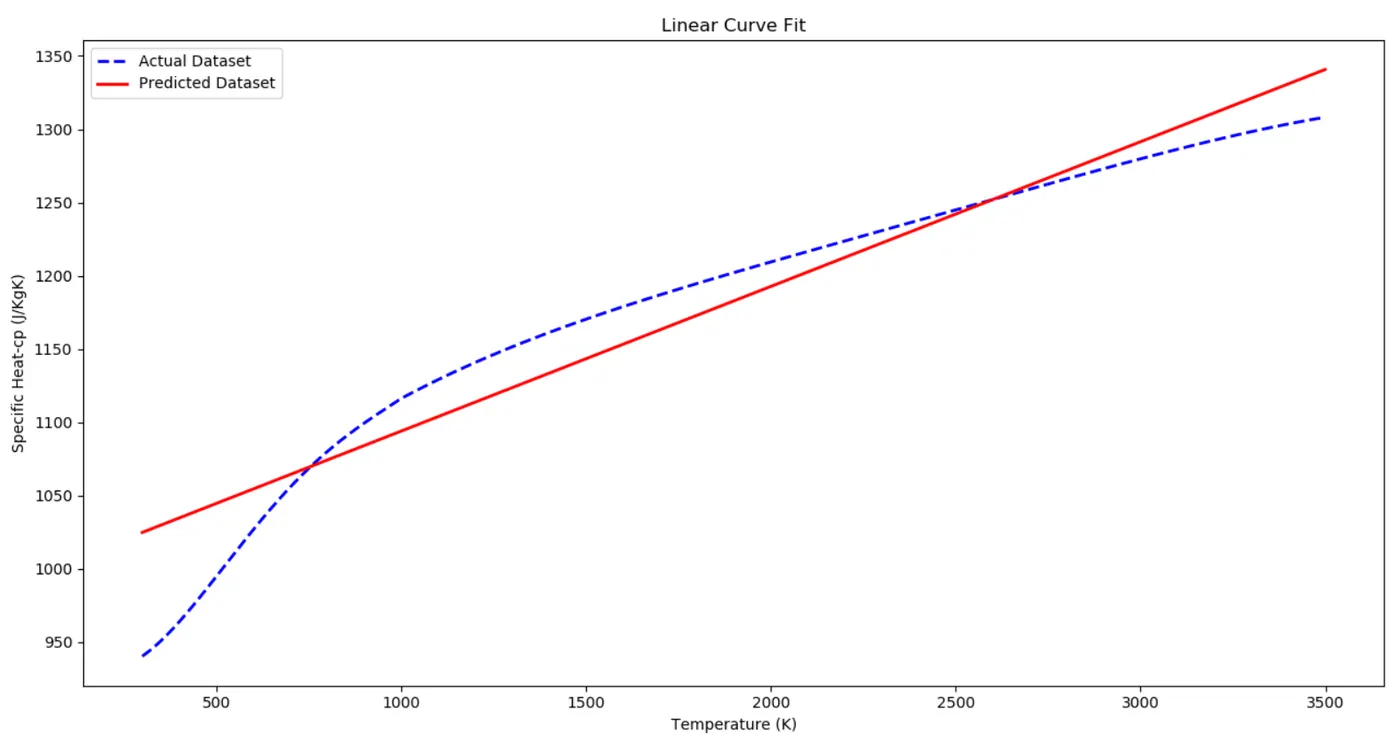
* From the above graph we can see the variation of the predicted Cp data with respect to the actual data.
* This is not the best fit as we have the so many mismatches in the curve and also the R^2 value is equal to '0.92' which is not that close to 1.
* The result for the fitness of the curve using linear function is found to be a good fit but not the best fit. This is verified using the plots made and by the R^2 method.
Cubic Curve fitting:
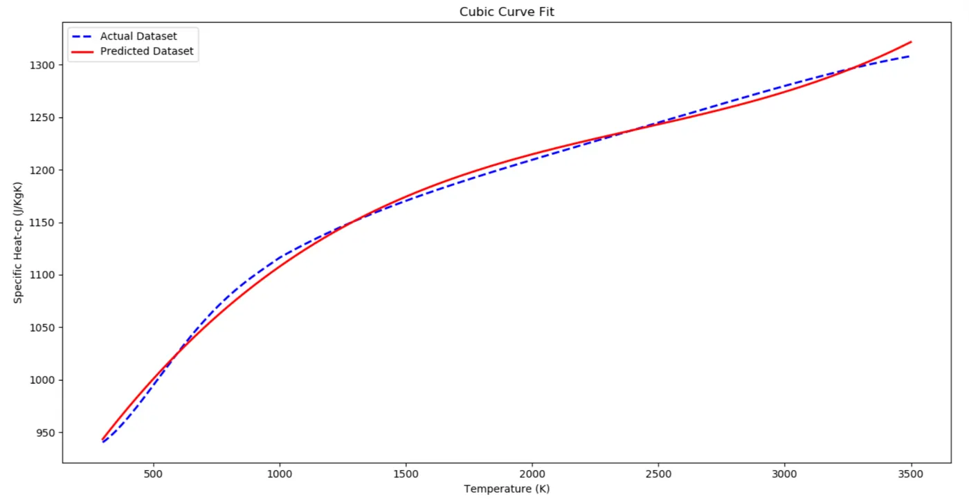
* From the above graph we can see the variation of the predicted Cp data with respect to the actual data.
* This is the best fit as we have less mismatches in the curve and also the R^2 value is equal to '0.99', which is very close to '1', and so this can be considered as the Best fit of the given dataset ito the function.
* Fitting the given data of Temperature & Cp in the Cubic Function is considered to have the Best fit and this is verified using the Plots made and by the R^2 method.

Finding Perfect Fit:
* To find the perfect fit, we need the R^2 value equal to 1, which says, all points lie exactly on the curve with no scatter. That means If you know X data points we can calculate the Y data point exactly, So the Curve variation can be calculated exactly for the future data points too.
* There are several ways to do that, one of the ways is using the scaling and centering process we can improve the cubic fit
* There is another method of splitting the dataset to find the predicted data with the independent variable (i.e) we can split the temperature range to 4 or 5 times and we can use diffrent order of the polynomial for fitting the data at each temperature range
* Here what we are doing this, we are increasing the order of the polynomial. When order of the polynomial is increased in the function the Predicted data of cp will be more accuarte and will match the actual dataset.
* For this we have changed the function defined to polynomial of order '5' (Quintic) & '8' (Octic), to measure the fitness of the curve.

Quintic curve fit:
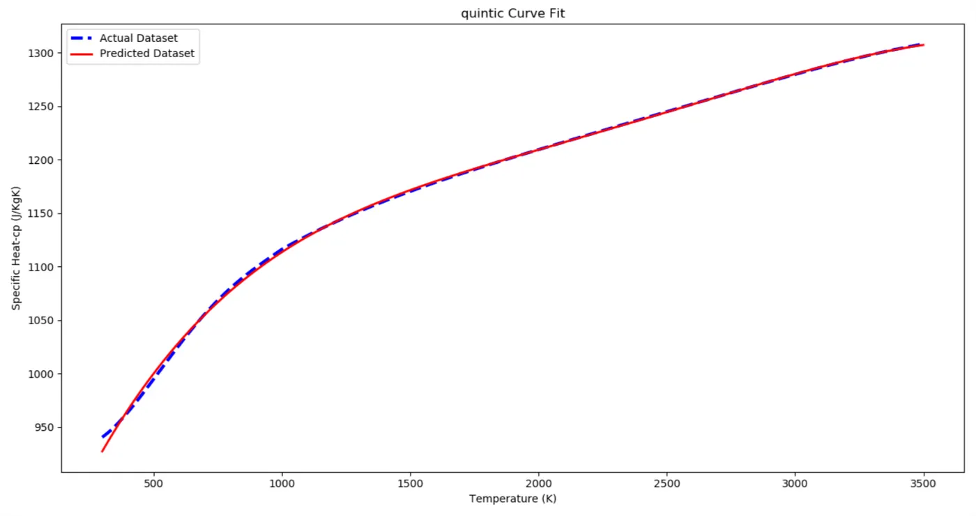
* This is a function of 5th degree polynomial and so from the plot we can see that, it is matching almost accurate to the actual dataset.
* From this we can say the fitness is getting better, with every increase in the order of the polynomial of the function we are defining.
* Still let us increase the order of polynomial to make the actual dataset and predicted dataset curves overlapping and to find more accurate fit.
Octic curve fit:
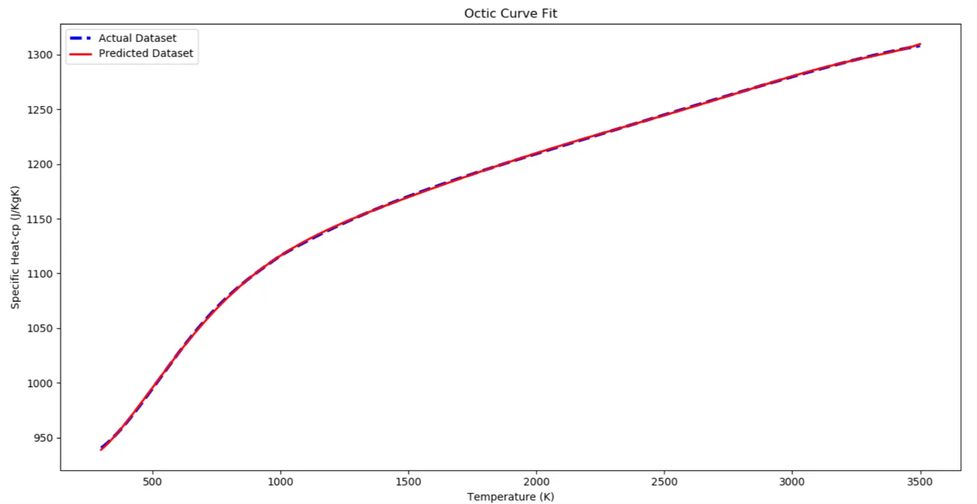
* This is a function of 8th degree polynomial and so from the plot we can see that, it is matching more accuratly to the actual dataset.
* Comparing the plots that we get for each function of increase in degree of polynomial we can say that, the fitness is getting better as the predicted dataset is found to overlap very closely to the actual dataset of Temperature and Cp.
* The R^2 value for Octic curve fit is even more close to 1 than the previous functions. From this we can say that, when the order of the polynomial increases the fit will move towards perfection and this can be clearly seen in the plots made and also by the method of R^2.
* Thus the curve fitting is done for the given data of Temperature & Cp using the linear & cubic functions. Also the fitness of the curve is measured using R^2 method. The fitness is improved by using Higher order function for the given dataset in the program and the fitness of the curves of each function defined is visualized using appropriate plots.