Week 5 - Curve fitting

1. AIM

To perform Curve Fitting for the given data containing temperature and Cp values using Python

2. METHODOLOGY

• What does popt and pcov mean?

Answer:

' popt ' refers to an array which consist of the coefficients of the polynomial specified at the begining of the program.

'pcov' refers to a square matrix which consist of the true variance and covariance of the parameters

• What does np.array(temperature) do?

Answer: np. array is used to create an array of temperature from the values stored in the data file using the numpy module.

• What does the * in *popt mean

Answer: * in *popt refers to te coefficients of the polynomial under consideration.

2.1 PYTHON CODE

import numpy as np 
import matplotlib.pyplot as plt 
from scipy.optimize import curve_fit
from statistics import mean 
import math

# Fourth order curve fit
def Quadratic_func(t,a,b,c,d,e):
	return a * pow(t,4) + b * pow(t,3) + c * pow(t,2) + d * t + e
# Third order curve fit	
def Cubic_func(t,a,b,c,d):
	return a * pow(t,3) + b * pow(t,2) + c * t + d

def linear_func(t,a,b):
	return a * t + b 

# Reading Input data file
def read_file():
	temperature = []
	cp = []
	for line in open('data','r'):
		values = line.split(',')
		temperature.append(float(values[0]))
		cp.append(float(values[1]))

	return[temperature, cp]

# Curve fit for linear equation
temperature, cp = read_file()
popt, pcov = curve_fit(linear_func, temperature, cp)
fit_cp = linear_func(np.array(temperature), *popt)
plt.plot(temperature, fit_cp, color = 'green', linewidth = 3)

# Curve fit for Qudratic equation (fourth order polynomial)
temperature,cp=read_file()
popt, pcov = curve_fit(Cubic_func, temperature, cp)
fit_cp = Cubic_func(np.array(temperature), *popt)
plt.plot(temperature, fit_cp, color = 'orange', linewidth = 3)
# Curve fit for Qudratic equation (fourth order polynomial)
temperature,cp=read_file()
popt,pcov=curve_fit(Quadratic_func,temperature,cp)
fit_cp=Quadratic_func(np.array(temperature),*popt)
plt.plot(temperature,fit_cp,color="red",linewidth=3)
plt.plot(temperature,cp,color="blue",linewidth=3)
plt.title('Specific Heat Vs Temperature')
plt.legend(['Linear Curve Fit','Cubic Curve Fit','Quadratic Curve Fit','Actual Data'])
plt.xlabel('Temperature[K]')	
plt.ylabel('cp')
plt.show()

# Goodness of fit - R_Square Calculation
def R_square(temperature,cp,fit_cp):
	for i in range(0,len(temperature)):
		Mean = mean(cp)
		SSR = np.sum(pow((fit_cp[i]-Mean),2))
		SSE = np.sum(pow((cp[i]-fit_cp[i]),2))
		SST = SSR+SSE
		R_2 = SSR/SST
	return R_2
temperature,cp=read_file()
R2 = R_square(temperature,cp,fit_cp)
print('fit value of Quadratic Curve is',R2)
print('Program end')

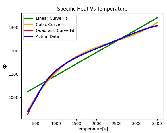
PLOT

OUTPUT

Inference: It is envisaged from the figure that as the order of the polynomial of the curve increases the curve fit is better. The fourth order polynomial/Quadratic Curve matches well with the actual data in comparison to the cubic curve which is in turn better when compared to linear curve. Furthermore, another method to improve the curve fit is by decreasing the element size or splitting the polynomial into a number of small curves to match the actual data.

3. CONCLUSION: The program to curve fit the given data was developed and executed successfully.