Week 5 - Curve fitting

OBJECTIVES :- To plot a best curve fitting by using linear, quadratic & cubic polynomial equations.

PROBLEM STATEMENTS :-

We have need to study on following problem statements-

1. What does popt and pcov mean?
2. What does np.array(temperature) do?
3. What does the *popt mean?
4. Write code to fit a linear and cubic polynomial for the Cp data. Explain if our results are good or bad.
5. What needs to be done in order to make the curve fit perfect?
6. Show empirically as to how well your curve has been fit.

CODE WITH EXPLAINATIONS :-

I created here three python codes for different equations as follows-

1. CODE FOR CURVE FITTING LINEAR EQUATIONS :-

import numpy as np
import matplotlib.pyplot as plt
from scipy.optimize import curve_fit

#curve fit function for linear equation
def func(t,a,b):
	return a*t + b

#reading thermodynamic data file
def read_file():
	temperature = []
	cp = []
	for line in open("data","r"):
		values = line.split(",")
		temperature.append(float(values[0]))
		cp.append(float(values[1]))

	return [temperature, cp]

#main program
temperature, cp = read_file()
popt,pcov = curve_fit(func, temperature, cp)
fit_cp = func(np.array(temperature), *popt)

sse = 0
for i in range(0,np.size(cp)):
	sse = sse + pow(cp[i] - fit_cp[i],2)
	print("For linear polynomial fit,")

#R_square
mean = np.sum(cp)/np.size(cp)
ssr = 0
for i in range(0, np.size(cp)):
	ssr = ssr + pow(fit_cp[i] - mean, 2)

sst = ssr + sse
R_square = ssr/sst
print("R_square = ", R_square)

plt.plot(temperature, cp,color = "blue", linewidth=3)
plt.plot(temperature, fit_cp, color = "red", linewidth = 3)
plt.legend(["Actual data","Curve fit"])
plt.xlabel("Temperature [K]")
plt.ylabel("Cp")
plt.savefig("Linear plot")
plt.show()

2. CODE FOR CURVE FITTING QUADRATIC EQUATIONS :-

import numpy as np
import matplotlib.pyplot as plt
from scipy.optimize import curve_fit

#curve fit function for quadratic equation
def func(t,a,b,c):
	return a*pow(t,2) + b*t + c

#reading thermodynamic data file
def read_file():
	temperature = []
	cp = []
	for line in open("data","r"):
		values = line.split(",")
		temperature.append(float(values[0]))
		cp.append(float(values[1]))

	return [temperature, cp]

#main program
temperature, cp = read_file()
popt,pcov = curve_fit(func, temperature, cp)
fit_cp = func(np.array(temperature), *popt)

sse = 0
for i in range(0,np.size(cp)):
	sse = sse + pow(cp[i] - fit_cp[i],2)
	print("For linear polynomial fit,")

#R_square
mean = np.sum(cp)/np.size(cp)
ssr = 0
for i in range(0, np.size(cp)):
	ssr = ssr + pow(fit_cp[i] - mean, 2)

sst = ssr + sse
R_square = ssr/sst
print("R_square = ", R_square)

plt.plot(temperature, cp,color = "blue", linewidth=3)
plt.plot(temperature, fit_cp, color = "red", linewidth = 3)
plt.legend(["Actual data","Curve fit"])
plt.xlabel("Temperature [K]")
plt.ylabel("Cp")
plt.savefig("Quadratic plot")
plt.show()

3. CODE FOR CURVE FITTING CUBIC POLYNOMIAL EQUATIONS :-

import numpy as np
import matplotlib.pyplot as plt
from scipy.optimize import curve_fit

#curve fit function for quadratic equation
def func(t,a,b,c,d):
	return a*pow(t,3) + b*pow(t,2) + c*t + d

#reading thermodynamic data file
def read_file():
	temperature = []
	cp = []
	for line in open("data","r"):			# r -> read the data file
		values = line.split(",")
		temperature.append(float(values[0]))
		cp.append(float(values[1]))

	return [temperature, cp]

#main program
temperature, cp = read_file()
popt,pcov = curve_fit(func, temperature, cp)
fit_cp = func(np.array(temperature), *popt)

# To check best or not curve fit
sse = 0
for i in range(0,np.size(cp)):
	sse = sse + pow(cp[i] - fit_cp[i],2)
	print("For linear polynomial fit,")

#R_square
mean = np.sum(cp)/np.size(cp)
ssr = 0
for i in range(0, np.size(cp)):
	ssr = ssr + pow(fit_cp[i] - mean, 2)

sst = ssr + sse
R_square = ssr/sst
print("R_square = ", R_square)

plt.plot(temperature, cp,color = "blue", linewidth=3)
plt.plot(temperature, fit_cp, color = "red", linewidth = 3)
plt.legend(["Actual data","Curve fit"])
plt.xlabel("Temperature [K]")
plt.ylabel("Cp")
plt.savefig("Cubic Polynomial plot")
plt.show()

1. Import numpy, matplotlib and curve_fit for creating list, plotting and linear curve.
2. Here has two functions, first for the equation and other one is for the thermodynamic data file.
3. Temperature is our input and Cp is our required output.
4. Read the data from data file (which provided in skill-lync challenge page) by seperating comma.
5. “0” is the first position where temperature value provided and “1” is a second position where Cp value is provided.
6. Return back same values upto final solutions.
7. Float function is provided because if there have intiger and decimal both the values then for getting both the values.
8. One things keep in mind that python code and data file must be kept in same folder for reading the file.
9. Write popt and pcov for getting best curve fit according to our functions.
10. Create temperature array w. r. t. variables (which are present in equations).
11. Now we need to check our curve fit is best or not for that write the code
12. Consider (sum of square of error) SSE = 0.
13. Put a for loop from range of zero to size of Cp.
14. Use the formula like “sse + (old_Cp - new_Cp)^2”
15. Square of this Cp because we need only positive values
16. Then go outside the loop and find out “mean = sum of Cp/size of Cp”
17. Consider (sum of square of regression) ssr = 0
18. Use for loop from zero to size of Cp
19. And then use the ssr formula like, “ssr = ssr + (new_Cp - mean)^2”
20. Then calculate sst by adding ssr and sse.
21. Also calculate R^2 = ssr/sst, to check curve is best or not.
22. Plots the graph temperature vs Cp and temperature vs fit_Cp(I.e. new_Cp).

DISCUSSIONS :-

I plot here three different graphs for three different equations as below-

1. CURVE FITTING PLOT FOR LINEAR EQUATION :-

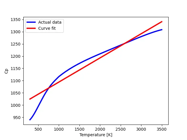
R_square = 0.924877

Red line shows that Curve fit while Blue line shows that Actual data given to us. From above figure we need to find out how & what much actual data is nearest to curve fit.

There have three range to define our results are good or bad as follows-

1. If R_square = 1, then our result is perfect
2. If R_square = 0.95 - 0.99, then our results is good
3. If R_square <= 0.94, then our results should be bad.

So, from these three conditions we can conclude that our results should be bad.

2. CURVE FITTING PLOT FOR QUADRATIC EQUATION :-

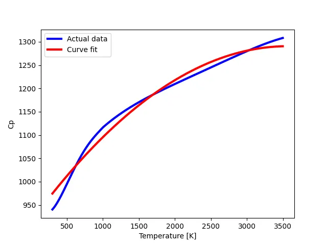
R_square = 0.98124

Red line shows that Curve fit while Blue line shows that Actual data given to us.

From above figure we see that curve fit line and actual data line are very nearer, it means there have less error. Also from our R-square value we can conclude that our results should be good because it is within range of 0.95 to 0.99. Also here has square of the error, so that we get less error and good curve.

3. CURVE FITTING PLOT FOR CUBIC POLYNOMIAL EQUATION :-

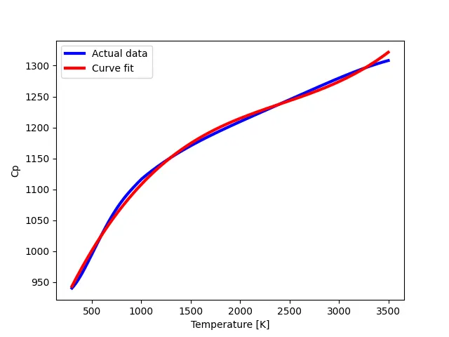
R_square = 0.996726

Red line shows that Curve fit while Blue line shows that Actual data given to us.

From above figure we can see that actual data line and curve fit line are very close to each other. It means there have very less error. Also from our R_square value we can conclude that our results should be best because it is more than 0.99. Here has the cube of error takesplace thats why we get very less error.

Now we can discuss about some questionary as follows-

Q.1.ANS:-

popt :- An array of optimal values for the parameters which minimizes the sum of square of residuals.

Pcov :- 2D array which contains the estimated co-varience of popt. The diagonal provides the variance of the parameter estimate.

Q.2.ANS:-

It gives the temperature list. It is the numpy module that’s why without importing this module we cant get list of temperature.

Q.3.ANS:-

It is the all functional variables reffer to the temperature here. Here, temperature gives those values which are reffer to the any one function.

Q.4.ANS:- The answer of this question with solutions I described above. As index of linear equation increases we get best curve fit means less error.

Q.5.ANS:- From above solutions if index of equation increases it means for higher order error is minimum because variable index reduces the error, it means we get best curve fit.

As R_square value increases we get best curve fit.

Q.6.ANS:- As empirically we can conclude that, as power of equation increases we get less error, because error decreases n-times and we get best curve fit. For details I describe everythings above with the help of plots.

CONCLUSIONS :-

From above python code and plots we can conclude that following points are-

1. For curve fitting plot we need three modules are numpy, matplotlib and curve fit.
2. Different order equation has different curve fitting.
3. If order of equation is lesser then we get more error and bad curve fitting and vice versa.
4. popt reffers variables of function and temperature vives value according to that.
5. R_square value showing the error of curve fitting and it shows the perfection of curve fitting plot.
6. One things keep in mind that, python code and data file must be in single folder.

In this way I calculate and explain everythings related to challenge and finally I concluded by analysing everythings and whole data.